HYPERLINK Function in Excel

If you want to create clickable links with a formula, you can use the HYPERLINK function in Excel. It can link to a web page, another sheet in your workbook, an email address, or a file on your computer.

Since a formula builds the link, the address can come straight from your data, and the link updates when that cell changes.

One catch: if you give it a whole column, it spills, but the labels and link formatting come out wrong. So you’ll use one formula per row and copy it down.

In this article, I’ll show you how to use HYPERLINK with six examples, including a clickable contents sheet and email links with a subject line.

HYPERLINK Function Syntax

Here is the syntax of the HYPERLINK function:

=HYPERLINK(link_location,[friendly_name])

• link_location – The address the link opens. It can be a web address, an email address, a file or folder path, or a place in the same workbook, typed in double quotes or taken from a cell.
• friendly_name – (Optional) The text or number the cell shows. It appears in blue and underlined, like any link.

If you leave out friendly_name, the cell shows the link_location itself. That’s fine for a short address, but a long web address fills the cell, so most of the time you’ll want a short label instead.

The HYPERLINK function works in Excel 365, 2024, 2021, 2019, 2016, Excel for Mac, and Excel for the web. In Excel for the web, it only works with web addresses (URLs).

When to Use the HYPERLINK Function

Use this function when you need to:

• Turn a column of web addresses into clickable links with readable labels
• Build a link from part of an address, like a product or movie ID
• Add a clickable contents sheet that jumps to other sheets in the workbook
• Create email links with the subject and message already filled in
• Open files in a folder without hunting for them in File Explorer
• Jump to a specific row in a long list

Let me show you a few practical examples of how to use the HYPERLINK function.

Example 1: Turn Web Addresses into Clickable Links

Let’s start with a simple one.

Below is a list of national parks with the web address of each park’s page, and I want a clickable link that shows the park’s name in column D.

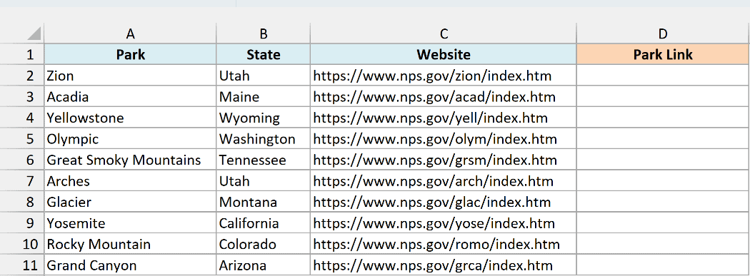
Here is the formula:

=HYPERLINK(C2,A2)

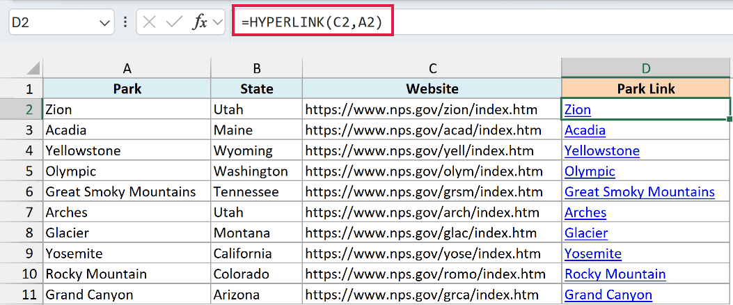
Enter it in cell D2 and copy it down to D11. Here, C2 is the link_location, so the link opens the park’s web page, and A2 is the friendly_name, so the cell shows Zion instead of the full address.

Important: Don’t give HYPERLINK the whole range in one formula, like =HYPERLINK(C2:C11,A2:A11). It spills ten links, but every cell shows the first park’s name and only the top cell looks like a link, so stick to one formula per row.

Once a cell holds a link, clicking it opens the link. To select the cell without opening the link (to copy or edit the formula, for example), click it and hold the mouse button until the pointer turns into a cross.

Example 2: Build a Link from an ID

Here’s another practical one, where your data only holds part of the address.

Below is a list of movies with each movie’s IMDb ID, and I want a link to the movie’s IMDb page in column D.

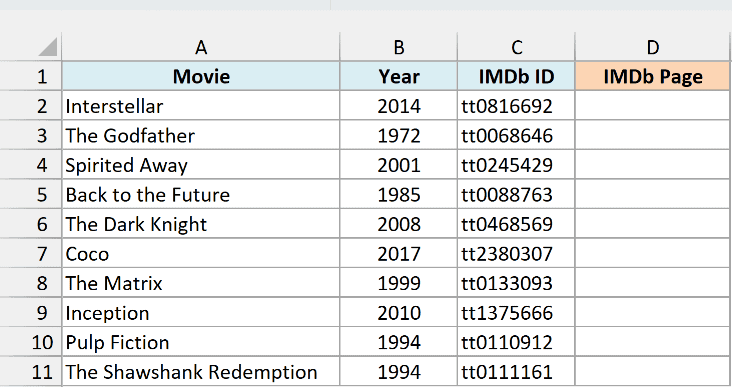
Here is the formula:

=HYPERLINK("https://www.imdb.com/title/"&C2,"Open on IMDb")

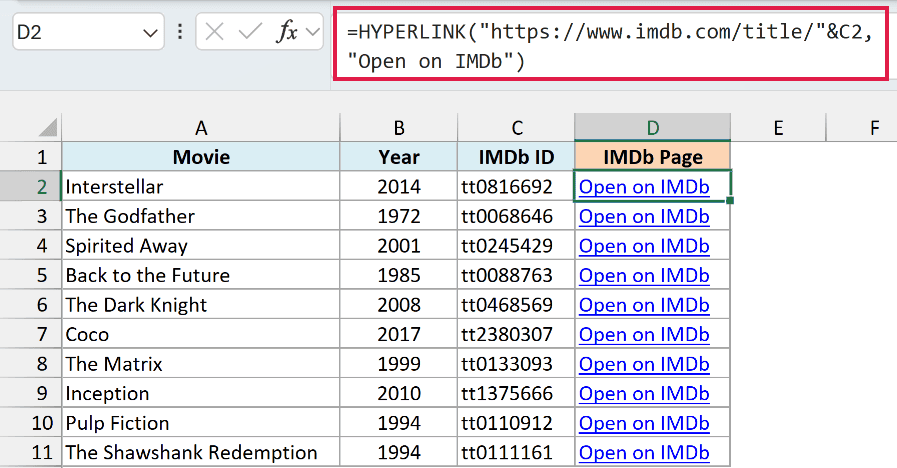
The formula joins the fixed start of the address (in double quotes) with the ID in C2, using the ampersand (&). So the link in D2 goes to https://www.imdb.com/title/tt0816692, the IMDb page for Interstellar.

The friendly_name is typed text this time, so every row shows the same Open on IMDb label. Each link still opens its own movie, because the ID in column C is different on every row.

The same idea works for any site whose addresses follow a pattern, like order tracking pages or product pages.

Example 3: Hyperlink to Another Sheet (Clickable Contents)

Now let’s use HYPERLINK to move around inside a workbook instead of opening a web page.

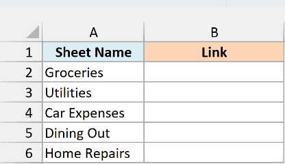
Below is a Contents sheet that lists five expense sheets in the same workbook (Groceries, Utilities, Car Expenses, Dining Out, and Home Repairs), and I want a link to each sheet in column B.

Here is the formula:

=HYPERLINK("#'"&A2&"'!A1","Go to "&A2)

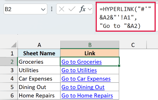
How this formula works:

• The # at the start tells Excel that the link goes to a place in this workbook, not to a web page or a file.
• The single quote right after the # and the one just before !A1 wrap the sheet name from A2, and !A1 is the cell the link lands on. So in B2, the full link_location is #’Groceries’!A1.
• “Go to “&A2 builds the label, so the cell shows Go to Groceries.

Important: The single quotes matter when a sheet name has a space in it, like Car Expenses. Without them, clicking the link does nothing and you stay on the Contents sheet.

Adding quotes around a name without a space, like Groceries, works fine too. That’s why one formula handles all five sheets.

It also helps to have a way back. Each expense sheet has a link in cell E1 that returns to the Contents sheet, and here is the formula in the Groceries sheet:

=HYPERLINK("#Contents!A1","Back to Contents")

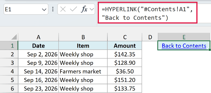
The sheet name Contents has no space, so it doesn’t need the single quotes. The same formula sits in E1 on all five expense sheets.

Example 4: Create an Email Link with a Subject and Message

This one is handy when you send the same kind of email to a lot of people.

Below is a list of swim club members with their email address and renewal date, and I want a link in column D that opens a ready-to-send renewal email for each member.

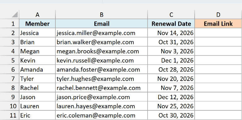
Here is the formula:

=HYPERLINK("mailto:"&B2&"?subject="&ENCODEURL("Membership renewal")&"&body="&ENCODEURL("Hi "&A2&", your swim club membership renews on "&TEXT(C2,"mmmm d")&"."),"Email "&A2)

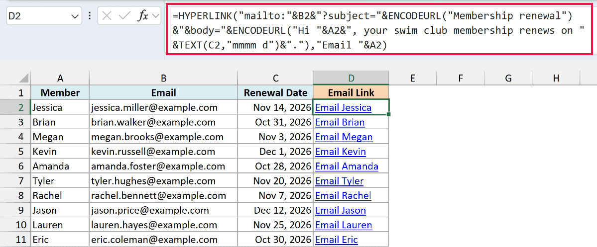
How this formula works:

• “mailto:”&B2 makes it an email link to the address in B2. Clicking it opens a new email in your default email app.
• ?subject= and &body= add the subject line and the message to that email.
• The ENCODEURL function converts the spaces and punctuation in your text into codes a link can carry, so a space becomes %20.
• TEXT(C2,”mmmm d”) turns the renewal date into words like November 14. Without it, the date would show up in the email as a number like 46340.
• “Email “&A2 is the label, so the cell shows Email Jessica.

The whole link_location can be at most 255 characters, including all the %20 codes, and a longer one shows a #VALUE! error. So keep the subject and message short.

Important: The ENCODEURL function only works in Excel for Windows. It isn’t available in Excel for Mac or Excel for the web, so this formula won’t work there.

If you are using Excel for Mac, you can use the SUBSTITUTE function to replace each space with %20 instead. Enter the below formula in cell D2 and then copy it down the range:

=HYPERLINK("mailto:"&B2&"?subject="&SUBSTITUTE("Membership renewal"," ","%20")&"&body="&SUBSTITUTE("Hi "&A2&", your swim club membership renews on "&TEXT(C2,"mmmm d")&"."," ","%20"),"Email "&A2)

Example 5: Open Files from a Folder

Let’s look at links that open files on your computer.

Below is a list of receipt PDFs saved in one folder, with the folder path in cell G1, and I want an Open receipt link for each file in column D.

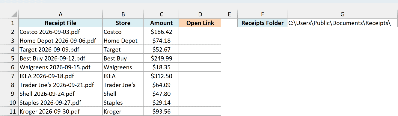
Here is the formula:

=HYPERLINK($G$1&A2,"Open receipt")

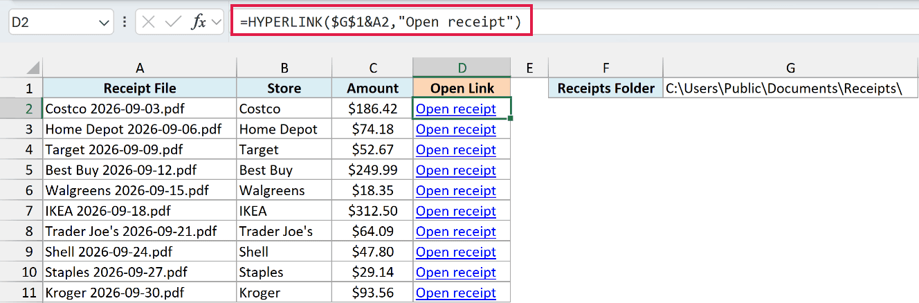
The formula joins the folder path in G1 with the file name in A2. So the link in D2 points to C:\Users\Public\Documents\Receipts\Costco 2026-09-03.pdf.

The $ signs lock the reference to G1, so every row uses the same folder as you copy the formula down. If you move the receipts to another folder later, you only change G1 and all ten links update.

The folder in this example is just a stand-in, so change G1 to the folder where your own files are. Clicking a link then opens that file, and if the file doesn’t exist, Excel shows an error message instead.

Important: Make sure the folder path in G1 ends with a backslash (\). Without it, the folder name and the file name run together, and none of the links can find their file.

Example 6: Hyperlink to the Cell with the First Match

Let’s step it up with a link that works out its own destination.

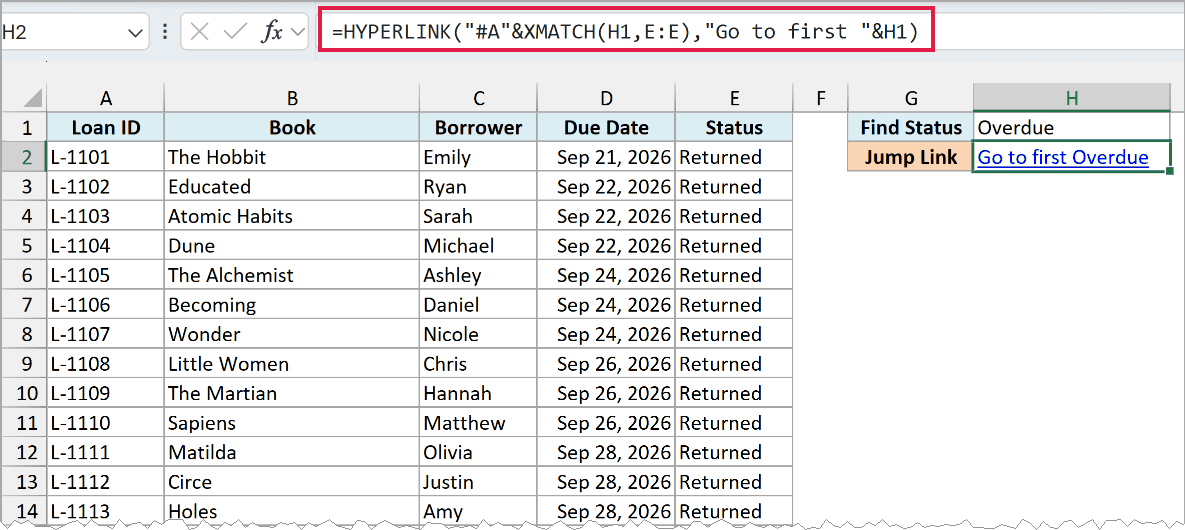
Below is a library loan list with 40 loans, and I want a link in H2 that jumps to the first loan with the status typed in H1.

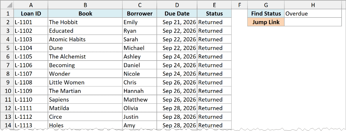
Here is the formula:

=HYPERLINK("#A"&XMATCH(H1,E:E),"Go to first "&H1)

How this formula works:

• XMATCH(H1,E:E) looks for Overdue in column E and returns its position, which is 32. Since the search starts at row 1, that position is also the row number.
• “#A”&32 becomes #A32. A # followed by just a cell address links to that cell on the same sheet.
• “Go to first “&H1 builds the label, so the cell shows Go to first Overdue.

When you click the link, Excel jumps down to cell A32, the first loan marked Overdue.

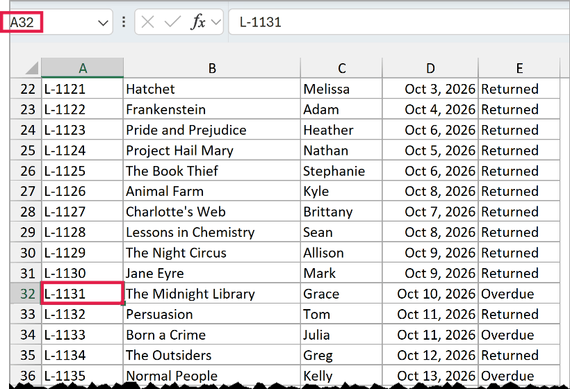
Change H1 to On Loan, and the same link now takes you to row 39. If H1 holds a status that isn’t in column E, Excel can’t find a match, so H2 shows #N/A instead of a link.

If you are using Excel 2019 or earlier, which doesn’t have the XMATCH function, enter the below formula in cell H2 instead:

=HYPERLINK("#A"&MATCH(H1,E:E,0),"Go to first "&H1)

So these are six ways to use the HYPERLINK function in Excel. I hope you found this tutorial useful.

List of All Excel Functions

Other Excel Articles You May Also Like:

• Create Dynamic Hyperlinks in Excel
• Extract URL from Hyperlinks in Excel
• How to Quickly Remove Hyperlinks from a Worksheet in Excel
• Hyperlinks in Excel (A Complete Guide + Examples)
• 20 Advanced Excel Functions and Formulas (for Excel Pros)
• How to Reference Another Sheet or Workbook in Excel (with Examples)