

The ACCRINT function calculates interest earned over a period for a security that pays interest regularly, such as a bond. This earned interest is called accrued interest.
You give it the dates, annual interest rate, face value, and payment schedule. It returns an interest amount in the same currency as the face value.
If an interest payment has already been made, the starting date matters. Calculating from the original issue date can include interest that was already paid.
ACCRINT needs a little care with ranges. In the Excel version tested here, a range passed directly returned an error; the examples below show how to convert the range so the results spill into separate cells.
Follow along with the example file
ACCRINT Function Examples.xlsx
ACCRINT Function Syntax
Here is the syntax of the ACCRINT function:
=ACCRINT(issue, first_interest, settlement, rate, par, frequency, [basis], [calc_method])
- issue: The date the security was issued. This is the starting date for the default interest calculation.
- first_interest: The first scheduled interest payment date. These periodic interest payments are also called coupons, and this date helps Excel establish the coupon schedule.
- settlement: The date the buyer takes ownership of the security. ACCRINT calculates accrued interest up to this date.
- rate: The annual coupon rate, entered as a percentage such as 6% or its decimal equivalent, 0.06.
- par: The security’s face value, such as 12000. This is the principal amount used to calculate interest, not its current market price.
- frequency: The number of coupon payments per year. Use 1 for annual, 2 for semiannual, or 4 for quarterly payments.
- basis: An optional code that tells Excel how to count days. It defaults to 0, and the five choices are listed below.
- calc_method: An optional calculation setting that defaults to TRUE, which calculates interest from issue to settlement. Microsoft documents FALSE as calculating from first_interest to settlement when settlement is after first_interest, but the tested result differs. Example 4 shows the discrepancy.
The day-count basis changes the fraction of a year used to calculate interest. Choose the convention specified for your security:
| Basis | Day-count convention |
|---|---|
| 0 or omitted | US (NASD) 30/360 |
| 1 | Actual/actual |
| 2 | Actual/360 |
| 3 | Actual/365 |
| 4 | European 30/360 |
The 30/360 conventions use adjusted 30-day months and a 360-day year, with different month-end rules for US and European methods. Actual/360 and actual/365 use elapsed calendar days, while actual/actual also considers the actual length of the coupon period.
If you leave the par argument empty between its commas, Excel uses 1,000. Supplying the face value explicitly makes it easier to check that you are calculating interest for the correct holding.
The ACCRINT function is available in desktop Excel 365, 2024, 2021, 2019, and 2016, including supported Mac editions. The spilling examples below need a version with dynamic arrays, such as Excel 365, 2024, or 2021.
When to Use the ACCRINT Function
Use this function when you need to:
- Calculate interest earned before a bond’s first coupon payment.
- Calculate accrued interest for several holding sizes of the same security.
- Check how a security’s day-count convention affects its accrued interest.
Let’s work through these calculations, then look at what happens when settlement falls after a coupon payment.
Example 1: Calculate Accrued Interest Before First Payment
Let’s start with one bond and one result. Below are the details of a $12,000 bond paying 6% annual interest, and we want its accrued interest on May 15, 2026, in cell B9.
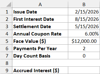
The bond was issued on February 15, 2026, and its first coupon is due on August 15. Since settlement is before that first payment, we are calculating interest earned from the issue date.
Enter this formula in cell B9:
=ACCRINT(B1,B2,B3,B4,B5,B6,B7)
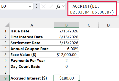
The result is $180.00. With basis 0, February 15 to May 15 counts as 90 days out of a 360-day year, so the calculation is $12,000 × 6% × 90/360.
The 2 in B6 tells Excel there are two coupon payments per year. The rate in B4 is still the annual 6%, so don’t halve it to 3% before using the function.
Dates stored as text can cause a #VALUE! error. Use real Excel dates in the input cells; the DATE function is one way to create them without relying on how Excel interprets a typed date.
The screenshots display dates as month/day/year. Your Excel settings may display the same dates differently, without changing the calculation.
Important: ACCRINT returns #NUM! if the issue date is on or after settlement, or the rate or face value is zero or negative. Also use the listed whole-number codes for frequency and basis.
Example 2: Calculate Interest for Several Holdings
Now suppose you hold different amounts of the same bond. Below are six face values with the same dates and coupon terms, and we want the accrued interest for each holding in column C.
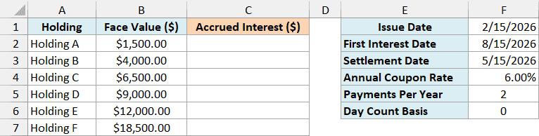
Enter this formula in C2:
=ACCRINT($F$1,$F$2,$F$3,$F$4,+B2:B7,$F$5,$F$6)
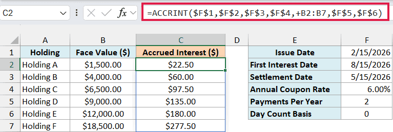
The formula returns six results, from $22.50 for Holding A to $277.50 for Holding F. Each holding earns 1.5% of its face value over this particular 90-day, basis-0 period.
The plus sign before B2:B7 matters. Passing B2:B7 directly returned #VALUE! in the tested Excel build; the unary + converts that reference into an array of values that ACCRINT can calculate together.
The dollar signs keep the shared inputs fixed, while the face-value array supplies one amount for each result. This setup works because all six holdings share the same security terms and settlement date.
The results spill from C2 into the cells below it. If those cells contain existing data, Excel can return #SPILL!, so clear the intended output cells before entering the formula.
For Excel 2019 or earlier, enter the following formula in C2 and copy it down to C7:
=ACCRINT($F$1,$F$2,$F$3,$F$4,B2,$F$5,$F$6)
This calculates one holding per row. The B2 reference changes as you copy down, while the shared inputs stay fixed.
Follow along with the example file
ACCRINT Function Examples.xlsx
Example 3: Compare Day-Count Bases
The same dates can produce different interest amounts when the day-count convention changes. Below are the five basis codes for the same $12,000 bond, and we want their accrued-interest results in column C.
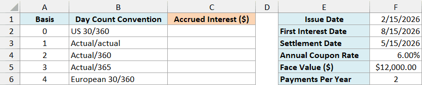
Enter this formula in C2:
=ACCRINT($F$1,$F$2,$F$3,$F$4,$F$5,$F$6,+A2:A6)
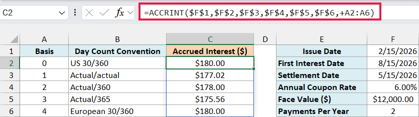
Here, the shared inputs stay fixed and the basis changes for each result. As in the previous example, the unary + converts the basis range into an array before passing it to ACCRINT.
Both 30/360 methods return $180.00 for these dates. They agree here because the dates don’t trigger a difference in their month-end adjustments; that does not mean the methods always give the same answer.
There are 89 actual days from February 15 to May 15, 2026. Actual/360 therefore returns $178.00, while actual/365 returns $175.56 because it divides those same 89 days by a larger denominator.
Actual/actual returns $177.02. The semiannual coupon is $360, and the full February 15 to August 15 coupon period has 181 days, so Excel allocates 89/181 of that coupon to the elapsed period.
The workbook shows currency with two decimal places. This number formatting changes how the result looks, while Excel retains the underlying value for later calculations.
Use the basis stated in the security’s terms. This comparison helps you see the effect of that choice; it isn’t a reason to select the method that produces the largest amount.
Example 4: Interest After a Coupon Payment
Once a coupon has been paid, interest since the original issue date can include interest that was already paid. If you need only the unpaid interest, you need to check where the calculation starts.
Below are a bond’s January 15 issue date, July 15 first coupon, and October 15 settlement, and we want to compare the calculation settings before finding interest since the last coupon in B12.
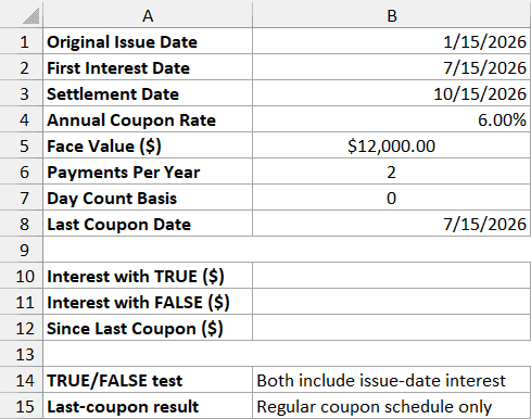
First, enter this formula in B10 with calc_method set to TRUE:
=ACCRINT(B1,B2,B3,B4,B5,B6,B7,TRUE)
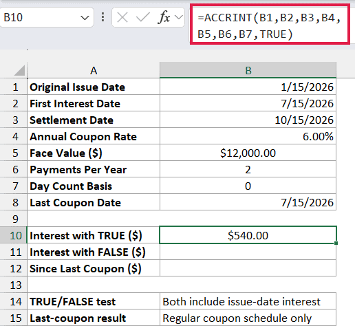
It returns $540.00, covering the 270 basis-0 days from January 15 to October 15. That includes the $360 coupon for January to July, even though the July payment date has passed.
Microsoft’s ACCRINT documentation says FALSE calculates from first_interest to settlement when settlement is later than first_interest. For these dates, that description would imply interest from July 15 to October 15.
Enter the FALSE version in B11 to compare it:
=ACCRINT(B1,B2,B3,B4,B5,B6,B7,FALSE)
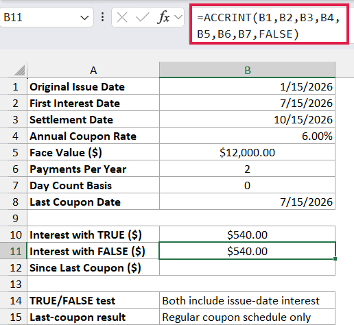
In Excel 16.0, build 20618, this also returns $540.00, not $180.00. The workbook records that observed result, so this example does not rely on FALSE to reset the calculation to the last coupon date.
For the regular coupon schedule shown here, the last coupon date is known: July 15, 2026, in B8. We can use that date for both date inputs at the start of the function to calculate just the current coupon period.
Enter this formula in B12:
=ACCRINT(B8,B8,B3,B4,B5,B6,B7)
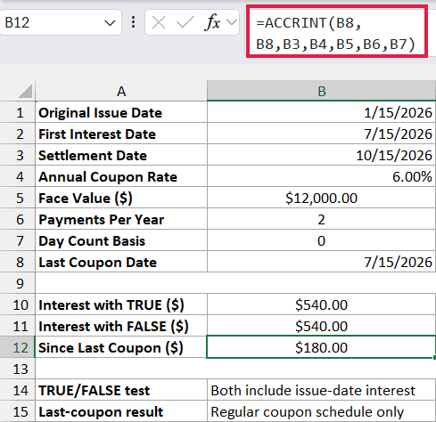
The result is $180.00, covering July 15 to October 15. The original issue date remains January 15; B8 is being used as the starting point for this calculation, not as a replacement historical issue date.
Important: This last-coupon calculation is for the regular coupon schedule shown, with a known previous coupon date. Don’t assume the same date substitution handles an unusually short or long first coupon period.
ACCRINT can calculate interest for one holding or a set of holdings, using the security’s dates and day-count basis. When a coupon date has passed, check that the result covers the interest period you actually need.
Other Excel Articles You May Also Like:
