

The ROMAN function in Excel converts numbers into Roman numerals, such as 4 into IV or 12 into XII. It saves you from typing those letter combinations yourself when you need Roman numeral labels.
In this tutorial, I’ll show you how to convert a list of numbers, compare Roman numeral styles, and create lowercase labels and year labels.
Follow along with the example file
ROMAN Function Examples.xlsx
ROMAN Function Syntax
Here is the syntax of the ROMAN function:
=ROMAN(number, [form])
- number (required): The number you want to convert. You can enter a number, refer to a cell, or supply a range of numbers in Excel versions that support dynamic arrays.
- form (optional): The Roman numeral style to use. Enter 0 for the classic style, 1 to 3 for progressively simplified styles, or 4 for the most simplified style.
When you leave out the form argument, Excel uses 0, the classic style. Changing the form changes how the Roman numeral is written, not the number it represents.
The form argument also accepts TRUE for the classic style and FALSE for the most simplified style. Example 2 shows the five numeric form choices side by side.
ROMAN works in Excel 365, 2024, 2021, 2019, 2016, Mac, and the web. The range formulas below need dynamic-array support in Excel 365, 2024, 2021, or the web; older-version alternatives are included.
When to Use the ROMAN Function
Use the ROMAN function when you need to:
- Turn chapter or section numbers into Roman numeral labels.
- Create lowercase Roman numerals for the opening pages of a document.
- Show a year in Roman numerals for an event or title.
Let me show you how these work in Excel.
Example 1: Convert Numbers to Roman Numerals
Let’s start with a list of numbers.
Below I have a list of chapter numbers, and I want to show their Roman numerals in column B.
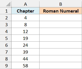
Enter the following formula in cell B2:
=ROMAN(A2:A9)
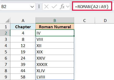
The formula converts each number in A2:A9 and fills B2:B9 automatically. This is called spilling, so you only need to enter the formula once.
For example, chapter 4 becomes IV, chapter 19 becomes XIX, and chapter 58 becomes LVIII. Since we haven’t supplied a form argument, all the results use the classic style.
If you get a #SPILL! error, make sure the cells below B2 are empty so Excel has room for all eight results.
Important: ROMAN returns text, so keep the original numbers for calculations. Use positive whole numbers from 1 to 3999 for your labels; an input such as -1 or 4000 returns a #VALUE! error.
If the input has a decimal part, ROMAN drops it instead of rounding it. For example, 14.9 becomes XIV, the Roman numeral for 14.
A zero or a reference to an empty cell returns empty text, so the result looks blank. Text that Excel can’t interpret as a number, such as “abc”, returns #VALUE!.
If you’re using Excel 2019 or earlier, enter the following formula in B2 and copy it down to B9:
=ROMAN(A2)
Example 2: Compare Roman Numeral Forms
Now let’s see what the optional form argument changes.
Below I have the five form choices and the number 2499 in cell E1, and I want to compare their Roman numerals in column B.
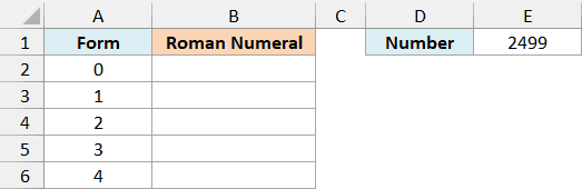
Enter the following formula in cell B2:
=ROMAN(E1,A2:A6)
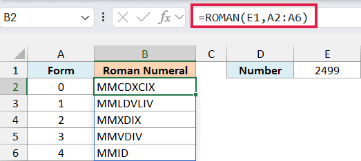
Here, E1 supplies the same number for every result, while A2:A6 supplies the five form choices. The formula spills one Roman numeral for each form.
With form 0, 2499 becomes MMCDXCIX. Form 4 shortens it to MMID, with the other forms producing the variations shown between them.
All five results represent 2499. The simplified forms use less familiar combinations, so leave the form argument out when you want the usual classic notation.
You can change E1 to compare a different number without editing the formula. Some numbers look the same in several forms, so don’t expect every form to produce a different result for every number.
Use one of the documented form choices, 0 through 4, TRUE, or FALSE. For example, a form value of 5 returns #VALUE!.
If you’re using Excel 2019 or earlier, enter the following formula in B2 and copy it down to B6:
=ROMAN($E$1,A2)
The dollar signs keep the number reference fixed on E1 as you copy the formula down.
Example 3: Create Lowercase Roman Numerals
Roman numerals for opening pages are often written in lowercase.
Below I have a list of opening sections and their page numbers, and I want lowercase Roman numeral labels in column C.
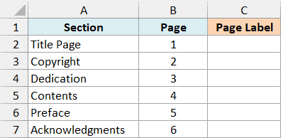
Enter the following formula in cell C2:
=LOWER(ROMAN(B2:B7))
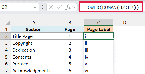
ROMAN first converts the page numbers into uppercase Roman numerals. The LOWER function then changes those letters to lowercase, giving us i through vi.
For example, the Contents page has page number 4, so its label is iv. Changing a page number updates its label automatically.
If you’re using Excel 2019 or earlier, enter the following formula in C2 and copy it down to C7:
=LOWER(ROMAN(B2))
Example 4: Show Years as Roman Numerals
You can also get a Roman numeral year from a date.
Below I have a list of events and their dates, and I want to show each event’s year in Roman numerals in column C.
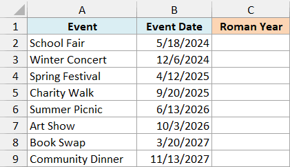
Enter the following formula in cell C2:
=ROMAN(YEAR(B2:B9))
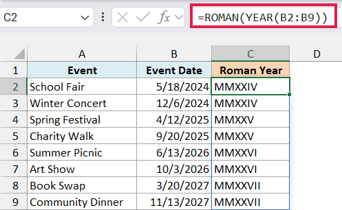
The YEAR function extracts the calendar year from each date, and ROMAN converts those year numbers into Roman numerals. For example, the Summer Picnic date is in 2026, so the result is MMXXVI.
The month and day don’t affect the result. Both events held in 2024 return MMXXIV, even though their dates are different.
Your dates may display differently depending on your regional settings, but that doesn’t change the year extracted from each date.
Important: Use real Excel dates in column B. Excel stores dates as serial numbers, so the YEAR function extracts the year before ROMAN converts it; passing the date directly would try to convert its serial number.
If you’re using Excel 2019 or earlier, enter the following formula in C2 and copy it down to C9:
=ROMAN(YEAR(B2))
In this tutorial, I showed you how to create Roman numeral labels, compare their forms, and use the LOWER and YEAR functions for lowercase labels and years.
To convert Roman numerals back into numbers, Excel has the ARABIC function. I hope you found this article helpful.
Other Excel Articles You May Also Like:
