

If you have text in mixed or messy capitalization and you want to turn it all into lowercase, the LOWER function is what you need. It takes whatever text you give it and returns the same text with every letter in lowercase.
In Excel 365, you can also feed LOWER a whole range and the results spill into the cells below, so one formula cleans up an entire column at once.
In this article, I’ll show you how to use LOWER with a few practical examples, from a basic conversion to building usernames and matching keys.
LOWER Syntax
Here is the syntax of the LOWER function:
=LOWER(text)
- text – The text you want to convert to lowercase. This can be a text string in quotes, a cell reference, or a range of cells in Excel 365.
Only letters are affected. Numbers, spaces, and punctuation are returned exactly as they were.
When to Use LOWER in Excel
Use the LOWER function when you need to:
- Clean up text that was typed in inconsistent capitalization
- Standardize values like email addresses so they all look the same
- Build lowercase usernames, handles, or URL slugs from names and titles
- Create a consistent key so records from different sources line up
Let me show you a few practical examples of how this works.
Example 1: Convert a Column of Text to Lowercase
Let’s start with the most basic use.
Below is a dataset with a list of product tags in column A. They were typed by different people, so the capitalization is all over the place.
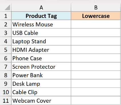
I want to convert this whole list to lowercase in one go.
Here is the formula:
=LOWER(A2:A11)
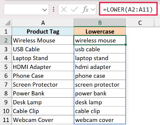
I entered this single formula in cell B2. Because it references the whole range A2:A11, the result spills down automatically and every tag comes back in lowercase.
Pro Tip: If you are on Excel 2019 or an older version, enter =LOWER(A2) in the top cell and drag it down the column instead. The spilling range version only works in Excel 365 and Excel 2021.
Example 2: Standardize Email Addresses
Here’s a common cleanup task.
Below is a signup sheet where people typed their own email addresses in column B. Some used capitals, some did not, so the same style of address looks different from row to row.
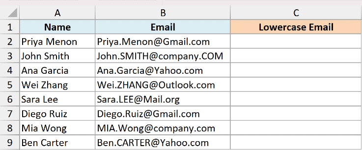
Email addresses are not case sensitive, so I want to store them all in clean lowercase.
Here is the formula:
=LOWER(B2:B9)
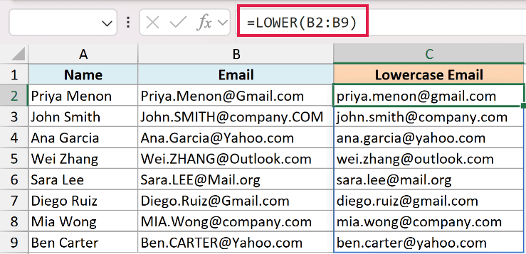
The formula converts every address to lowercase in one spill. Now the list is consistent and ready to paste back or send to another system.
Example 3: Build Lowercase Usernames and Handles
Now let’s combine LOWER with another function.
Below is a list of employee full names in column A. I want to turn each one into a lowercase username with no spaces.
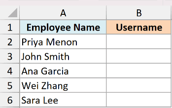
First I want a plain handle, so I need to drop the space between the first and last name and lowercase everything.
Here is the formula:
=LOWER(SUBSTITUTE(A2," ",""))
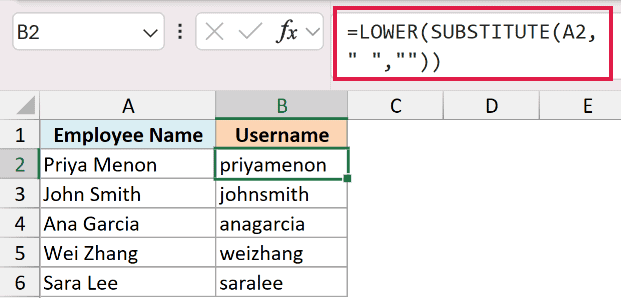
Here is how this formula works:
- SUBSTITUTE removes the space by replacing it with nothing, so “Priya Menon” becomes “PriyaMenon”.
- LOWER then converts that result to lowercase, giving “priyamenon”.
Sometimes you want a URL slug instead, where the space becomes a hyphen rather than disappearing.
Here is the formula for that:
=LOWER(SUBSTITUTE(A2," ","-"))
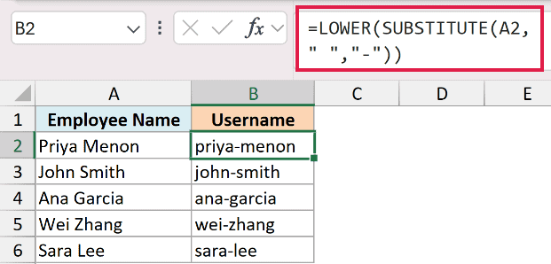
This time SUBSTITUTE swaps the space for a hyphen, so “Priya Menon” comes out as “priya-menon”, which is the kind of clean handle you would use in a link.
Example 4: Create a Consistent Key to Match Two Lists
Here’s a scenario I run into a lot when combining data from different places.
Below are two company names in columns A and B that should refer to the same records, but the capitalization does not match (“Apple Inc” versus “APPLE INC”).
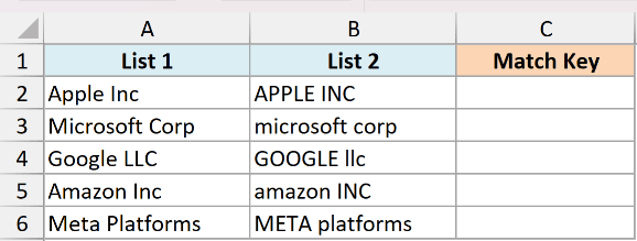
I want a clean lowercase version of column A that I can use as a matching key.
Here is the formula:
=LOWER(A2)
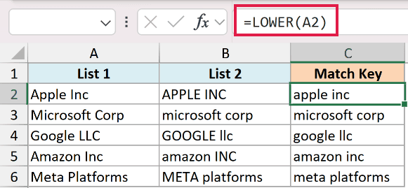
This gives me a single lowercase form of each name. When I do the same to the other list, both sides use identical text and line up cleanly.
Excel’s own lookups like VLOOKUP and COUNTIF already ignore case. This lowercase key matters when the data leaves Excel, for example a Power Query merge, a database import, or a join with another tool, where “Apple Inc” and “APPLE INC” would not match.
Example 5: Compare Two Columns Ignoring Case
Let’s finish with a comparison.
Below are two columns of product codes that came from two different systems. I want to check whether each pair is the same, treating capitalization differences as a match.
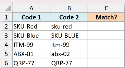
I want a TRUE or FALSE result showing whether the codes match once case is ignored.
Here is the formula:
=LOWER(A2)=LOWER(B2)
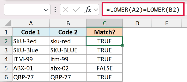
Both codes are lowercased first, then compared. So “SKU-Red” and “sku-red” return TRUE, while a genuinely different code returns FALSE.
Pro Tip: The = operator is already case insensitive, so =A2=B2 gives the same result here. LOWER earns its place when you need a case sensitive function to ignore case instead, such as EXACT, where =EXACT(LOWER(A2),LOWER(B2)) confirms a match without caring about capitalization.
Tips & Common Mistakes
- Numbers and symbols are left alone. LOWER only changes letters, so a value like “Order #A100” becomes “order #a100”. The digits, the hash, and the space stay exactly as they were.
- The result is text, not the original cell. LOWER returns a new value in a separate cell. To replace the originals, copy the formula results and use Paste Special > Values over the source column, then delete the helper formulas.
- Empty cells return empty text. Running LOWER on a blank cell returns an empty string rather than a zero, so you will not get stray 0s in your cleaned column.
- LOWER does not remove extra spaces. It only changes case. If your text also has messy spacing, wrap it in TRIM as well, like =LOWER(TRIM(A2)).
That covers the main ways to use the LOWER function in Excel. It only does one job, changing letters to lowercase, but that one job comes up a lot when you are standardizing emails, building usernames, or cleaning up data before a match.
If you work with text case often, the UPPER and PROPER functions work the same way for uppercase and title case.
Other Excel Articles You May Also Like:
