

If you have text that was typed in a mix of upper and lower case and you want it all in capital letters, the UPPER function is the quickest way to do it.
You hand it some text, and it hands back the same text with every letter turned into a capital. In Excel 365, you can also feed UPPER a whole range and the results spill into the cells below.
In this article, I’ll show you how to use UPPER in Excel, from a simple one-column conversion to cleaning up messy imported data and building consistent codes.
UPPER Function Syntax
Here is the syntax of the UPPER function:
=UPPER(text)
- text – The text you want converted to uppercase. This can be text typed in directly (in quotes), a cell reference, or a range of cells.
UPPER only changes letters. Any numbers, spaces, and symbols in the text are left exactly as they are.
UPPER works in every version of Excel, including Microsoft 365, Excel 2024, 2021, 2019, and older versions, plus Excel on the web.
When to Use UPPER in Excel
Use the UPPER function when you need to:
- Convert names, titles, or labels to all capital letters
- Standardize codes and abbreviations (like state or currency codes) that people typed inconsistently
- Clean up text pulled in from another system before you use it
- Build consistent product codes or keys where the case has to match
Let me show you a few practical examples of how this works.
Example 1: Convert a Column of Text to Uppercase
Let’s start with the simplest case.
Below is a list of product names in column A. They were typed in a mix of cases, and some include model numbers.
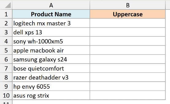
I want all of these names in uppercase in column B.
Here is the formula:
=UPPER(A2:A10)
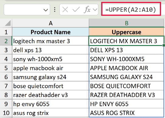
I entered the formula once in cell B2 and pointed it at the whole range A2:A10. In Excel 365, the results spill down the column automatically, so there is no need to copy the formula to each row.
Notice that the numbers in the model names (like the 3 in “MX Master 3”) stay exactly as they were. UPPER only touches the letters.
Pro Tip: If you are on Excel 2019 or earlier, dynamic arrays are not available. Enter =UPPER(A2) in the first cell instead and copy it down the column.
Example 2: Standardize State and Currency Codes
Here’s a common cleanup job.
Below is an orders table where someone entered the state code in column A and the currency code in column B. The cases are all over the place (“ca”, “Tx”, “usd”, “Eur”).
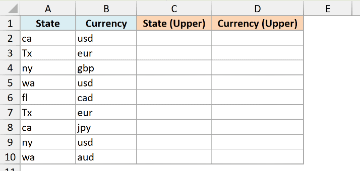
I want both codes in clean uppercase so they are consistent for filtering and reports.
Here is the formula:
=UPPER(A2:B10)
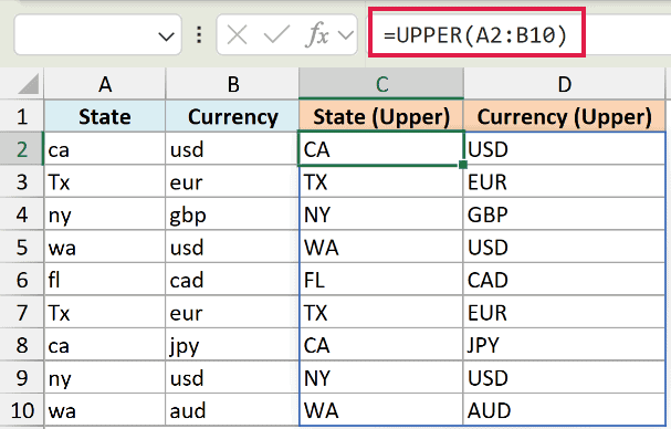
Because I pointed UPPER at both columns at once, it spills a matching two-column block of clean codes. Every code now reads the same way regardless of how it was originally typed.
This matters more than it looks. A PivotTable or a filter treats “ca” and “CA” as the same label, but a person scanning the report does not. Consistent case keeps your data readable and export-ready.
Example 3: Clean and Uppercase Imported Data
Here’s a combination I reach for a lot.
When you pull data from another system, you often get extra spaces along with mixed case. Below is a list of member IDs in column A with stray spaces before, after, and inside some of them.
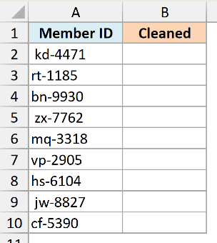
I want each ID trimmed of extra spaces and converted to uppercase in one step.
Here is the formula:
=UPPER(TRIM(A2:A10))
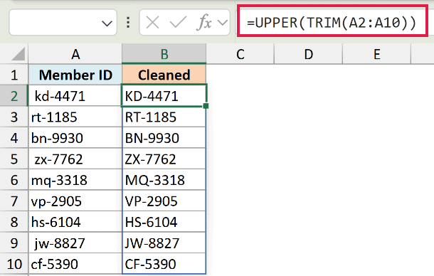
Here, the TRIM function runs first and strips out the leading, trailing, and double spaces. UPPER then takes that cleaned-up text and capitalizes it.
Nesting the two means you fix the spacing and the case with a single formula, instead of using a helper column for each. The TRIM function is handy any time imported text looks clean but refuses to match other values.
Example 4: Build Uppercase Product Codes (SKUs)
This next one is something I use quite often.
Below I have a product category in column A and a numeric ID in column B. I want to turn them into a single uppercase SKU like “ELE-1024”.
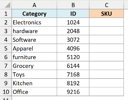
I want to take the first three letters of the category, add a dash, then the ID, all in uppercase.
Here is the formula:
=UPPER(LEFT(A2,3)&"-"&B2)
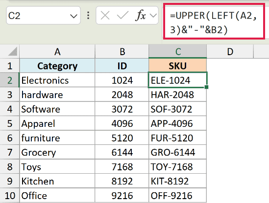
How this formula works:
- LEFT(A2,3) pulls the first three letters of the category (for example, “Ele” from “Electronics”).
- &”-“&B2 joins that to a dash and the numeric ID.
- UPPER(…) wraps the whole thing so the result comes out in capitals, giving you “ELE-1024”.
Because the case is now fixed, every SKU you generate looks identical in style. That consistency also helps when you later match these codes against another list.
Example 5: Uppercase an Entire Table at Once
Let’s finish with the dynamic array way of handling a whole table.
Below is a small table with first names, last names, and cities across columns A to C, again in mixed case.
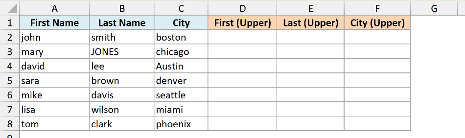
Instead of writing a formula for each column, I want to convert the entire table to uppercase with one formula.
Here is the formula:
=UPPER(A2:C8)
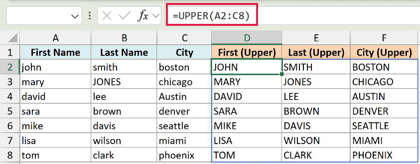
I entered this once in cell E2, and it spills the whole three-column block into E2:G8 in uppercase. The shape of the output matches the shape of the input range.
This is the cleanest way to uppercase a block of data in Excel 365. In older versions you would need one formula per cell, filled across and down.
Tips & Common Mistakes
- UPPER only changes letters. Numbers, spaces, punctuation, and symbols pass through untouched, so it is safe to run on codes and IDs that mix letters and digits.
- UPPER creates a new result, it does not edit the original. To replace the original text, copy the formula cells, then use Paste Special and choose Values over the original column before deleting the formulas.
- There is no keyboard shortcut for changing case in Excel. Unlike Word (Shift + F3), Excel has no built-in shortcut, so UPPER, Flash Fill, or a macro is the way to do it.
- Use the right function for the job. UPPER capitalizes everything. If you only want each word to start with a capital, that is PROPER, and if you want everything in small letters, that is LOWER.
Wrapping It Up
The UPPER function is a small tool that solves a very common problem: text that was typed inconsistently. Wrap a cell or a whole range in UPPER and you get clean, all-caps text back in seconds.
Once you combine it with functions like TRIM, LEFT, and the ampersand, you can clean, standardize, and build codes without ever retyping anything by hand.
Other Excel Articles You May Also Like:
