

The COUPNCD function returns a bond’s next coupon payment date after settlement. A coupon is the bond’s regular interest payment, and settlement is the date the purchase is completed.
You give Excel the settlement date, maturity date, and number of payments per year. It finds the next date on that payment schedule, including when settlement falls on a coupon date or the schedule runs into February.
Follow along with the example file
COUPNCD Function Examples.xlsx
COUPNCD Function Syntax
Here is the syntax of the COUPNCD function:
=COUPNCD(settlement, maturity, frequency, [basis])
- settlement: The date the bond purchase is completed. Excel uses this as the starting point for finding the next coupon date.
- maturity: The date the bond’s principal (the amount borrowed) is due to be repaid. Together with frequency, this determines the regular coupon schedule.
- frequency: The number of coupon payments per year. Use 1 for annual, 2 for semiannual (every six months), or 4 for quarterly payments.
- basis: Optional. A number from 0 to 4 specifying the day-count convention, which is the rule used to count days in bond calculations. Leaving it out uses 0, or US 30/360.
The basis choices are 0 for US 30/360, 1 for actual/actual, 2 for actual/360, 3 for actual/365, and 4 for European 30/360. Use the convention specified for the bond; values outside this range return a #NUM! error.
Excel truncates all four arguments to integers. A decimal frequency such as 2.9 is treated as 2, so enter the intended whole-number frequency and basis rather than relying on that conversion.
COUPNCD works in Excel 365, 2024, 2021, 2019, and 2016. The spilling examples below use dynamic arrays; each also includes a fill-down formula for Excel 2019 and earlier.
When to Use the COUPNCD Function
Use COUPNCD when you need to:
- Add the next scheduled interest payment date to a bond tracker.
- Compare the next coupon dates for bonds with different payment frequencies.
- Check how the next payment date changes when settlement is on a coupon day or near the end of February.
Let’s work through these using the four sheets in the example file.
Example 1: Find the Next Coupon Date
Below are the details of a bond bought on February 10, 2026, with two coupon payments per year, and we want its next coupon date in cell B6.
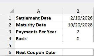
Enter this formula in B6:
=COUPNCD(B1,B2,B3,B4)
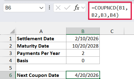
The result is April 20, 2026. The bond matures on October 20, 2028, and pays twice a year, so its regular coupon dates fall on April 20 and October 20.
COUPNCD picks the first of those dates after the February 10 settlement. It doesn’t add six months to the settlement date, which would put the result in August instead.
If B6 shows a number, select it and choose Short Date from the Number Format dropdown on the Home tab. Excel stores dates as numbers, and you can change the date format to control how you see them.
The screenshots use month/day/year. Your date display may look different because of your regional settings or the format you choose.
Both input dates must be real Excel dates. Unrecognized date text can produce #VALUE!, while a settlement date on or after maturity produces #NUM! because there isn’t a later coupon date within the bond’s term.
Example 2: Compare Different Payment Frequencies
Below is a list of six bonds with different settlement dates, maturity dates, and payment frequencies, and we want each next coupon date in column E.
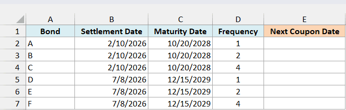
In Excel with dynamic arrays, enter this formula in E2:
=COUPNCD(+B2:B7,+C2:C7,+D2:D7)
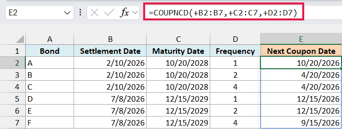
The formula spills six results down column E. Each row uses its own settlement date, maturity date, and frequency, and the omitted basis defaults to 0.
The plus signs matter here. COUPNCD can reject a multi-cell reference with #VALUE!; putting + before each range passes its numeric values as an array so Excel can calculate a result for each row.
For the first three bonds, annual payments give October 20, 2026, while semiannual and quarterly payments both give April 20, 2026. Different payment frequencies can still have the same next coupon date.
The last three rows show a different outcome: annual and semiannual payments both give December 15, 2026, while quarterly payments give September 15, 2026. In each case, the maturity date anchors the schedule.
Frequency means payments per year, so use 2 for a six-month interval, not 6. Values other than 1, 2, or 4 return #NUM! after Excel truncates any decimal part.
Keep the cells below E2 clear so the results have room to spill. If a cell is occupied, Excel shows #SPILL! instead of filling the result range.
For Excel 2019 or earlier, enter this formula in E2 and copy it down through E7:
=COUPNCD(B2,C2,D2)
Each copied formula calculates one bond’s date, so it doesn’t need the plus signs.
Example 3: Settlement on a Coupon Date
The word “next” matters when settlement falls on a payment day.
Below are settlement dates just before, on, and after a bond’s coupon dates, and we want to compare the next payment dates in column B.
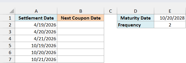
Enter this formula in B2:
=COUPNCD(+A2:A7,$E$1,$E$2)
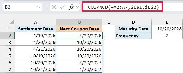
The formula uses each settlement date in column A with the maturity date and frequency stored in E1 and E2. As in the previous example, + converts the settlement range into an array of values.
For settlement on April 19, the next coupon date is April 20, 2026. Move settlement forward one day to April 20, and the result becomes October 20, 2026.
COUPNCD returns a coupon date strictly after settlement. It skips the coupon on the settlement date itself, which is also why an October 20 settlement returns April 20 of the following year.
For Excel 2019 or earlier, enter this formula in B2 and copy it down through B7:
=COUPNCD(A2,$E$1,$E$2)
The dollar signs keep the shared maturity and frequency references fixed as the settlement reference moves down.
Example 4: February and Leap-Year Coupon Dates
A coupon schedule tied to the end of August needs a little care when the other payment falls in February.
Below are settlement dates for a bond that matures on August 31, 2028, and pays twice a year, and we want its next coupon dates in column B.
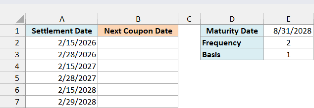
Enter this formula in B2:
=COUPNCD(+A2:A7,$E$1,$E$2,$E$3)
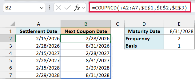
Here, E3 supplies basis 1, or actual/actual. The formula uses the same maturity date and payment frequency for all six settlements and spills the next coupon dates down column B.
For settlement on February 15, the next coupon falls on February 28 in 2026 and 2027. In 2028, a leap year, the result is February 29.
This bond’s semiannual schedule lands on the last day of February and August. COUPNCD handles the different February lengths, so you don’t need to hard-code the 28th or add a leap-year check.
The rows that settle on the February coupon date return August 31 of the same year. That follows the same strictly-after rule from the previous example.
For Excel 2019 or earlier, enter this formula in B2 and copy it down through B7:
=COUPNCD(A2,$E$1,$E$2,$E$3)
These examples show how COUPNCD finds the next coupon date for a single bond or a list of bonds. The settlement-day and February examples help you check the dates that are easy to get wrong when building a schedule manually.
Other Excel Articles You May Also Like:
