

The DETECTLANGUAGE function in Excel identifies the language of text and returns its language code, such as en for English or fr for French.
When you have messages in several languages, those codes give you a way to organize them before deciding which ones to translate. The function uses Microsoft’s online translation service, so you need an internet connection.
In this tutorial, I’ll show you four examples, including checking a list of messages, keeping blank rows empty, showing language names, and filtering out English text.
Follow along with the example file
DETECTLANGUAGE Function Examples.xlsx
DETECTLANGUAGE Function Syntax
Here is the syntax of the DETECTLANGUAGE function:
=DETECTLANGUAGE(text)
- text – Required. The text you want to identify, or a reference to the cell or range containing it.
When you type text directly into the argument, put it in double quotes. When the text is already in a cell, use its reference without quotes.
You can also supply a range of text cells. Excel returns a separate language code for each cell, as the first example shows.
DETECTLANGUAGE is available in Excel for Microsoft 365 on Windows and Mac, and in Excel Mobile. The examples below use Microsoft 365 for Windows.
When to Use the DETECTLANGUAGE Function
Use this function when you need to:
- Identify the languages in a list of messages or notes.
- Show readable language names alongside text.
- Separate messages by language before reviewing or translating them.
Let me show you how these work in Excel.
Example 1: Detect Languages in a List
Let’s start with the function on its own.
Below is a list of hotel guest requests, and I want to identify each request’s language in column B.
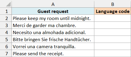
Enter this formula in cell B2 on the Example 1 sheet:
=DETECTLANGUAGE(A2:A7)
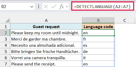
The formula checks each request in A2:A7 and spills six language codes into B2:B7. You enter it once in B2, so there’s no need to copy it down.
The results are en, fr, es, de, it, and en. These stand for English, French, Spanish, German, Italian, and English, in the same order as the requests.
For example, “Necesito una almohada adicional.” returns es. DETECTLANGUAGE identifies the language but leaves the original message unchanged.
Make sure the cells below B2 are empty before entering the formula. If something is blocking the result area, Excel can return a #SPILL! error instead of showing the codes.
Important: DETECTLANGUAGE needs Microsoft’s online service. You may briefly see #BUSY! while it gets the results, so wait for the language codes before using them in another task.
Microsoft also applies a daily usage quota. If Excel reports that the request was throttled, you’ve reached that limit and need to try again later; Microsoft doesn’t give a numeric quota on the function’s documentation page.
Because this is an online service, supported languages and detection results can change over time.
Example 2: Keep Blank Rows Empty
Some lists have gaps where no one entered a message.
Below are library notes with two empty rows, and I want the language codes in column B while keeping those rows blank.
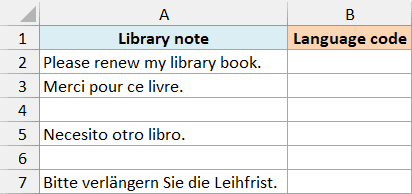
Enter this formula in B2 on the Example 2 sheet:
=IF(A2:A7="","",DETECTLANGUAGE(A2:A7))
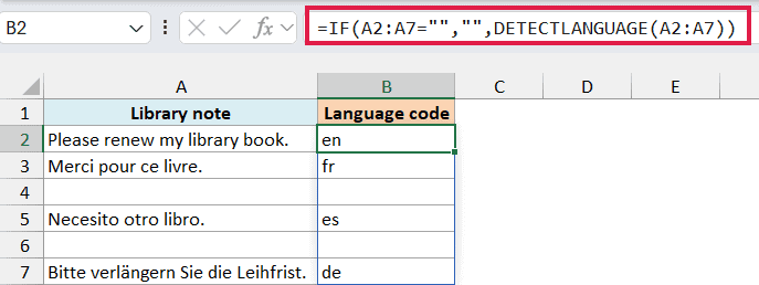
The IF function checks whether each input equals an empty string. For those rows, it returns "", which looks blank; for the other rows, it returns the detected language code.
Here, B4 and B6 stay visually blank because A4 and A6 are empty. The other results are en, fr, es, and de, alongside their corresponding notes.
The empty-looking results are still part of the spill, so you can’t type over B4 or B6 individually. Edit the source note in column A to change its result.
This check handles empty cells and formulas returning an empty string. A cell containing spaces isn’t empty, and a number or date isn’t valid text for DETECTLANGUAGE.
If a cell contains a very long passage and Excel reports that the text is too long, shorten the text you submit. The blank check doesn’t hide text-length errors or service failures.
Example 3: Show Full Language Names
A language name is easier to read than a code when you share a worksheet.
Below are comments from a book club, and I want to show each comment’s language name in column B.
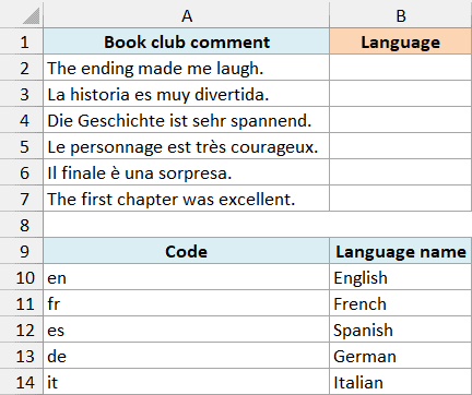
The small lookup table below the comments pairs five language codes with their names. Enter this formula in B2 on the Example 3 sheet:
=XLOOKUP(DETECTLANGUAGE(A2:A7),A10:A14,B10:B14,"Unlisted code")
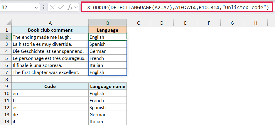
This returns English, Spanish, German, French, Italian, and English for the six comments.
How this formula works:
DETECTLANGUAGE(A2:A7)returns a language code for each comment.- The XLOOKUP function finds each code in A10:A14 using its default exact match.
- It returns the corresponding name from B10:B14. If a detected code isn’t in the table, it returns “Unlisted code”.
The lookup table only covers the five languages used here. If you add other languages, extend the table and both lookup ranges in the formula; Microsoft’s language-code list can help you match the codes.
“Unlisted code” means the code is missing from your lookup table. It doesn’t mean the service failed to identify the language, and it doesn’t replace a service error.
Example 4: Filter Out English Messages
You can also use the detected language to decide which messages appear in a separate list.
Below are messages about evening classes, and I want to list only the non-English messages in column C.
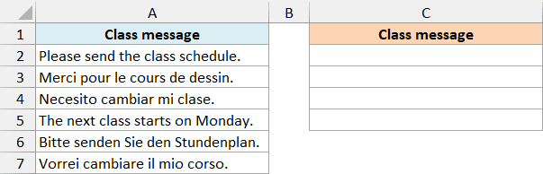
Enter this formula in C2 on the Example 4 sheet:
=FILTER(A2:A7,DETECTLANGUAGE(A2:A7)<>"en","No messages")
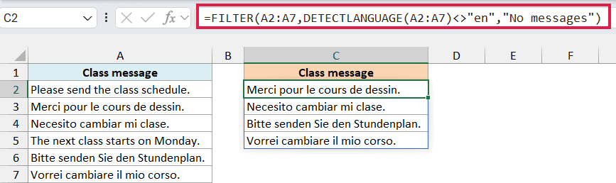
The four French, Spanish, German, and Italian messages appear in C2:C5. The two English messages stay in the source list but don’t appear in the filtered results.
How this formula works:
DETECTLANGUAGE(A2:A7)identifies the language of each message.<>"en"means “not equal to en”, so it returns TRUE for messages detected as a language other than English.- The FILTER function returns the messages whose test is TRUE. If none qualify, it displays “No messages”.
This example uses nonblank text in every source row. If detection returns an error for any message, that error can also stop the filtered list from returning results.
For one small list, putting detection inside the filter keeps the formula compact. If you need to inspect or reuse the codes for several tasks, keep a separate language-code column like the one in Example 1.
Important: Very short or mixed-language text can be ambiguous. Review uncertain messages before relying on the filtered list, because a detected code is the service’s classification of the text.
These examples show how to identify languages, turn codes into readable names, and select messages by their detected language. To change the text into another language, use the TRANSLATE function.
Other Excel Articles You May Also Like:
