

The ODD function in Excel takes a number and rounds it up to the next odd whole number, like 3, 5, or 7. If the number is already odd, ODD leaves it alone.
You’ll want it whenever an even number would cause a problem, like a vote that could end in a tie or a layout that needs one item right in the middle.
Below, I’ll walk you through five examples, including a formula for the nearest odd number and a fix for blank cells.
Follow along with the example file
ODD Function Examples.xlsx
ODD Function Syntax
Here is the syntax of the ODD function:
=ODD(number)
- number – The value you want to round up to an odd number. It can be a typed number, a cell reference, or a calculation, and in Excel 365 or Excel 2021 and later, it can also be a whole range.
ODD always rounds away from zero. So a negative number gets more negative, which means -2 becomes -3 and -5.1 becomes -7.
Zero isn’t an odd number, so =ODD(0) returns 1. An odd whole number, positive or negative, comes back exactly as it is.
The ODD function works in Excel for Microsoft 365, Excel 2024, 2021, 2019, and 2016, on both Windows and Mac.
When to Use the ODD Function
Use this function when you need to:
- Make a group size odd so a vote or a match can’t end in a tie
- Plan a layout with one item right in the center, like a row of tiles
- Arrange plants or decorations in odd-numbered groups
- Round the result of a calculation up to the next odd number
Let me show you a few practical examples of how to use the ODD function.
Example 1: Round Up to the Next Odd Number
Let’s start with a simple example.
Below is a game night list with the number of rounds each pair of players asked for, and since a match with an odd number of rounds can’t end in a tie, I want the rounds to play in column C.
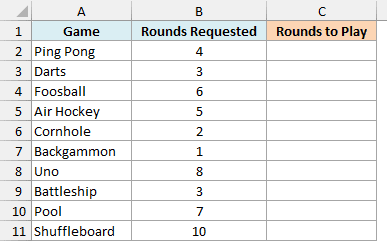
Here is the formula:
=ODD(B2:B11)
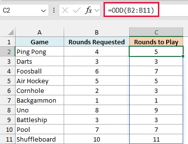
ODD goes through the requests in B2:B11 and bumps every even number up by one. Ping Pong asked for 4 rounds, so it gets 5, while Darts asked for 3 and keeps 3 because it’s already odd.
You enter the formula once in C2, and it spills the results for all ten games down to C11. If something is already sitting in C3:C11, the formula shows a #SPILL! error instead, so keep that range clear.
If you are using Excel 2019 or earlier, enter the below formula in cell C2 and then copy it down the range:
=ODD(B2)
The same goes for every spilling formula in this article. Point it at the first cell of the range, then copy it down.
Example 2: Round Decimals Up to an Odd Number
Now let’s see how ODD handles decimals.
Below is a list of rooms with the width of each one in feet, and since I’m laying 1-foot tiles with one tile centered in each room, I want the number of tiles across each room in column C.
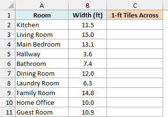
Here is the formula:
=ODD(B2:B11)
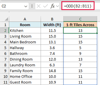
A centered layout has one middle tile plus the same number of tiles on each side, so the count across is always odd. ODD gives you that count by rounding each width up to the next odd number.
The Kitchen is 11.5 feet wide, so it needs 13 tiles across, with the tiles at each wall cut to fit. Whole numbers work just like in Example 1, so the 12-foot Dining Room also gets 13, and the 15-foot Living Room stays at 15.
Now look at the Main Bedroom. At 13.1 feet, it’s only a tenth of a foot wider than 13, but ODD skips 14 because it’s even and lands on 15.
That’s the right count for the tiles, too. The extra tenth of a foot leaves a thin gap at each wall, and each of those gaps needs its own cut tile.
Important: A value that displays as 13 but is really 13.0000001 (common when it comes from another calculation) also becomes 15. If that happens, round the value before ODD sees it, like =ODD(ROUND(B2,2)), which returns 13.
Example 3: Round a Calculated Result Up to an Odd Number
Here’s a scenario where the number you need to round comes from a calculation.
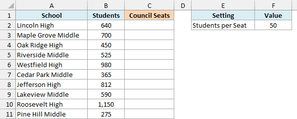
Below is a list of schools with the number of students in each, and I want the student council seats for each school in column C, at one seat for every 50 students (the value in F2).
Here is the formula:
=ODD(B2:B11/F2)
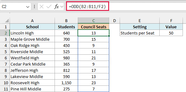
The B2:B11/F2 part divides each school’s student count by 50. For Lincoln High, that’s 640 divided by 50, which is 12.8 seats.
ODD then rounds that up to an odd number, so Lincoln High gets 13 seats. With an odd number of seats, a yes-or-no vote where every member votes can’t end in a tie.
Maple Grove Middle shows what happens with a whole number. Its 700 students give exactly 14 seats, but since 14 is even, ODD returns 15.
Because the 50 sits in its own cell, you can change F2 to a different number of students per seat, and every school’s seat count updates.
If you are using Excel 2019 or earlier, enter the below formula in cell C2 and then copy it down the range:
=ODD(B2/$F$2)
The dollar signs lock the reference to F2, so it doesn’t shift as you copy the formula down.
Example 4: Round to the Nearest Odd Number in Excel
ODD only ever rounds up. When you want the closest odd number instead, you need a small formula.
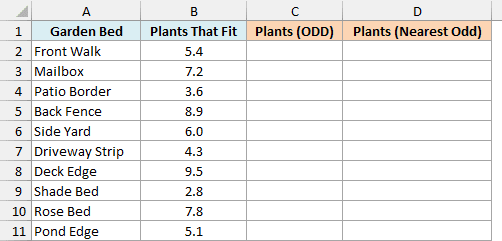
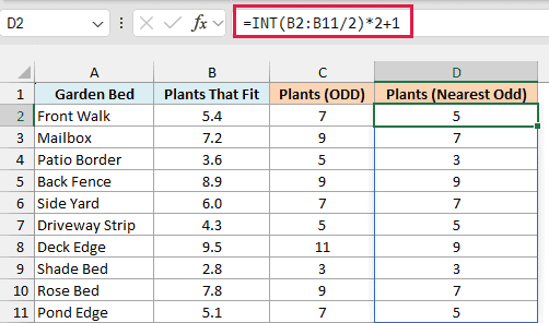
Below is a list of garden beds with how many plants fit in each at the recommended spacing, and since odd groups look more natural, I want the number to plant using ODD in column C and the nearest odd number in column D.
Here is the ODD formula for column C:
=ODD(B2:B11)
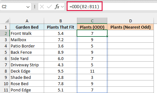
ODD rounds every value up, so the Front Walk, where 5.4 plants fit, gets 7. That’s almost two plants more than the bed has room for.
And here is the formula for the nearest odd number in column D:
=INT(B2:B11/2)*2+1
How this formula works:
- B2:B11/2 halves each value, so the Front Walk’s 5.4 becomes 2.7.
- The INT function drops the decimal part, which leaves 2.
- Multiplying by 2 gives the even number at or just below the original value, which is 4.
- Adding 1 gives the odd number right above it, which is 5.
Every value sits between two even numbers, like 5.4 between 4 and 6. The odd number in that gap, 5 here, is always the closest odd number, and that’s the one this formula returns.
Compare the two columns for the Deck Edge. ODD turns its 9.5 into 11, while the nearest odd number is 9.
The Side Yard’s 6.0 sits exactly halfway between 5 and 7. In that case the formula picks the higher one, so both columns give 7.
The nearest odd number can still go a little over what fits (the Driveway Strip’s 4.3 becomes 5). But it’s never more than one plant away, while ODD can add almost two.
If you are using Excel 2019 or earlier, enter the below formula in cell D2 and then copy it down the range:
=INT(B2/2)*2+1
You might also see =EVEN(B2)-1 suggested for this. It gives the same answer for most positive numbers, but it breaks on negative ones (-3.2 becomes -5 instead of -3), so I stick with the INT version.
Example 5: Handle Blank Cells and Text With the ODD Function
This last one is about messy data, which is where ODD can quietly give you a wrong answer.
Below is an RSVP list for an office awards dinner with the guests from each team, team lead included, and I want the number of seats for each table in column D.
Each team lead sits in the middle of the table with the same number of people on each side, so every table needs an odd number of seats.
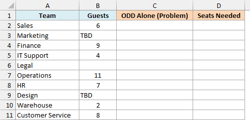
First, let’s see what a plain ODD formula does with this data in column C:
=ODD(B2:B11)
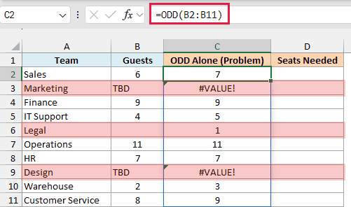
The TBD entries for Marketing and Design return the #VALUE! error, because ODD can’t round text. These errors also break anything built on the results, so a total like =SUM(C2:C11) returns #VALUE! too.
The bigger problem is Legal. Its Guests cell is empty, but ODD returns 1, because Excel reads a blank cell as 0 and ODD rounds 0 up to 1.
That 1 looks like a real reply, so you could end up setting a table for a team that hasn’t answered yet. Unlike an error, it doesn’t stand out, which makes it easy to miss.
Here is the formula that fixes both problems in column D:
=IF(ISNUMBER(B2:B11),ODD(B2:B11),"")
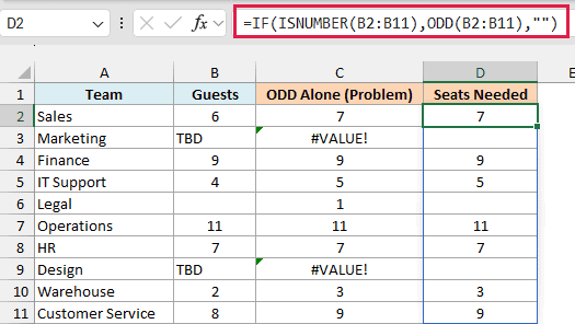
The ISNUMBER function checks each cell in B2:B11 and returns TRUE only when it holds a number. IF then runs ODD on those cells and returns an empty text string for everything else, so the TBD rows and Legal’s blank row stay empty.
With both problems fixed, =SUM(D2:D11) returns 51 seats.
If you are using Excel 2019 or earlier, enter the below formula in cell D2 and then copy it down the range:
=IF(ISNUMBER(B2),ODD(B2),"")
Note that a guest count stored as text, like “8”, would also be left empty, because ISNUMBER doesn’t treat it as a number. If your list has numbers stored as text, convert them to real numbers first.
So these are five ways to use the ODD function in Excel. It only takes one argument, but keep an eye on decimals, which always jump up, and blank cells, which turn into 1.
If you need even numbers instead, the EVEN function works the same way.
And if you only want to check whether a number is odd, the ISODD function returns TRUE or FALSE. It works on one cell at a time, though, and returns #VALUE! if you give it a range like B2:B11.
I hope you found this article helpful.
Other Excel Articles You May Also Like:
