

The PDURATION function in Excel tells you how many periods it takes for an amount to grow from where it is today to a target value, at a fixed growth rate.
It’s handy for questions like “how many years until my savings hit $25,000?” or “how long does it take to double my money at 8%?”. You give it the rate, the starting value, and the target, and it does the compounding math for you.
In this article, I’ll show you how PDURATION works, starting with a single investment and moving on to monthly compounding, target years, and growth that isn’t money at all. I’ll also cover the cases PDURATION can’t handle and what to use instead.
Follow along with the example file
PDURATION Function Examples.xlsx
PDURATION Function Syntax
Here is the syntax of the PDURATION function:
=PDURATION(rate, pv, fv)
- rate – the growth or interest rate per period
- pv – the present value, which is the amount you’re starting with
- fv – the future value, which is the target amount you want to reach
All three arguments are required.
The result is a number of periods, and the period is whatever your rate is based on. A yearly rate gives you years, and a monthly rate gives you months.
Enter the rate as a percentage, like 5% or 0.05. If you type 5 instead, Excel reads it as 500%, and you get a tiny result that looks fine but is completely wrong.
All three arguments must be greater than zero. A zero or negative value (or a blank rate cell) returns the #NUM! error, and text that isn’t a number returns #VALUE!.
The PDURATION function works in Excel 2013 and later on Windows, including Excel for Microsoft 365, 2024, 2021, 2019, and 2016, and in Excel for Microsoft 365, 2024, and 2021 on Mac.
When to Use the PDURATION Function
Use this function when you need to:
- Find how many years a one-time deposit takes to reach a savings goal
- Compare how long different goals, rates, or rising costs (like rent) take
- Work out how long it takes to double an investment
- Estimate when a growing number (revenue, subscribers, users) will hit a target
Let me show you a few practical examples of how to use the PDURATION function.
Example 1: Find How Many Years an Investment Takes to Reach a Target
Let’s start with a simple example.
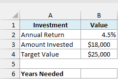
Below I have the details of a one-time investment of $18,000 that earns 4.5% a year, and I want to find how many years it will take to grow to $25,000 in cell B6.
Here is the formula:
=PDURATION(B2,B3,B4)
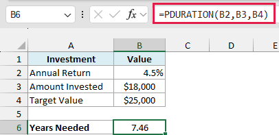
The formula returns 7.46, which means the investment needs about 7.46 years at 4.5% a year to grow from $18,000 to $25,000.
In the above formula, B2 is the annual return, B3 is the amount invested, and B4 is the target value. Since the rate is a yearly rate, the answer is in years.
Note that PDURATION assumes the rate stays the same every year and that you don’t add or take out any money along the way. It works with a single lump sum growing on its own.
Example 2: Find When Rent Will Hit Your Budget in Several Cities
Now let’s do the same thing for a whole list in one go, and with something that isn’t an investment.
Below is a list of cities with the yearly rent increase, the current rent, and a budget limit, and I want to find how many years until the rent in each city reaches that limit in column E.
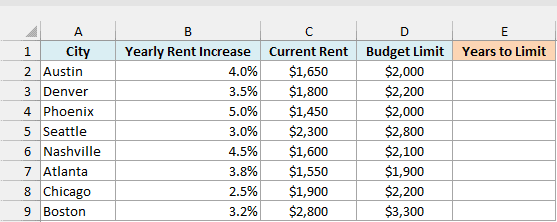
Here is the formula:
=PDURATION(B2:B9,C2:C9,D2:D9)
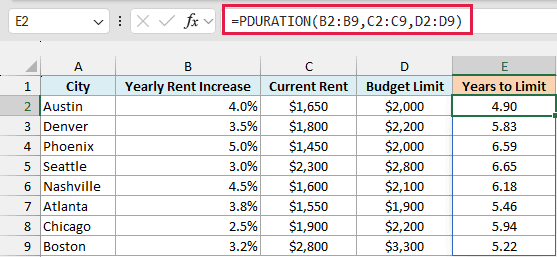
Instead of one cell for each argument, this formula gives PDURATION the whole increase, rent, and limit columns. It returns one result per row, and these results spill into E2:E9 on their own.
For example, Austin and Seattle both need their rent to go up by about 21% to hit the limit. Austin gets there in 4.90 years at 4% a year, while Seattle takes 6.65 years at 3% a year.
If you are using Excel 2019 or earlier, enter the below formula in cell E2 and then copy it down to E9:
=PDURATION(B2,C2,D2)
Example 3: Find How Long It Takes to Double Your Money
Now let’s use PDURATION to answer a classic money question.
Below I have a list of interest rates, and I want to find how many years it takes to double money at each rate in column B.
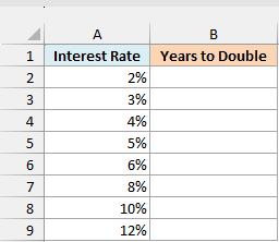
Here is the formula:
=PDURATION(A2:A9,1,2)
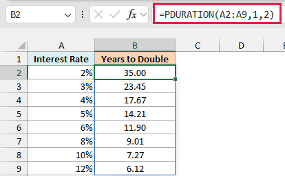
Here, I’ve used 1 as the present value and 2 as the future value. Doubling is the same whether you start with $1 or $10,000, because PDURATION only cares about how many times bigger the target is than the starting amount.
The results show that money takes 35 years to double at 2%, about 9 years at 8%, and a little over 6 years at 12%.
Pro Tip: You may have heard of the Rule of 72, where you divide 72 by the interest rate to estimate the doubling time. At 8%, it gives 72/8 = 9 years, and PDURATION gives the exact answer, 9.01.
If you are using Excel 2019 or earlier, enter the below formula in cell B2 and then copy it down to B9:
=PDURATION(A2,1,2)
Example 4: Get the Result in Months (Monthly Compounding)
Now let’s look at an account where interest is added every month instead of every year.
Below are the details of a high-yield savings account that pays 4.8% a year, compounded monthly, and I want to find how many months it takes to grow from $6,500 to $8,000 in cell B7.
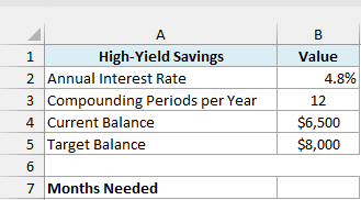
Here is the formula:
=PDURATION(B2/B3,B4,B5)
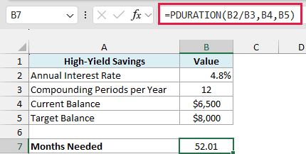
The formula returns 52.01, so the balance reaches $8,000 in a little over 52 months (about 4 years and 4 months).
The key part here is B2/B3. Since the interest is added 12 times a year, I divide the annual rate of 4.8% by 12 to get the monthly rate (0.4%).
Because the rate is now monthly, PDURATION returns the answer in months.
Important: Always use the rate for one compounding period. If you use the annual 4.8% here, you get 4.43 years, and multiplying that by 12 gives 53.15 months, not 52.01, because it assumes interest is added only once a year.
PDURATION can’t handle regular deposits. If you plan to add, say, $200 every month on top of the starting balance, use the NPER function instead, since it accepts a regular payment.
Example 5: Find the Year a Revenue Goal Will Be Reached
You can use PDURATION for business numbers too, as long as they grow at a steady rate.
Below I have a bakery’s revenue for the current year and its expected yearly growth, and I want to find the number of years needed to reach $500,000 in cell B7 and the year it happens in cell B8.
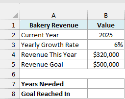
Here is the formula that gives the years needed:
=PDURATION(B3,B4,B5)
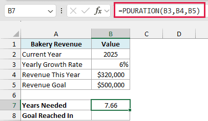
This returns 7.66 years. But the bakery measures revenue once a year, so 7.66 isn’t a year you can actually point to.
After 7 years at 6%, revenue would be about $481,000, which is still short of the goal. It’s only after the 8th year that it crosses $500,000.
Here is the formula that gives the year the goal is reached:
=B2+ROUNDUP(B7,0)
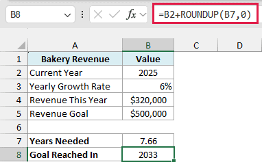
The ROUNDUP function turns 7.66 into 8 full years, and adding that to the current year in B2 (2025) gives 2033.
Use ROUNDUP here and not the ROUND function. ROUND would turn something like 7.3 years into 7, which is one year before the goal is actually reached.
Example 6: Use PDURATION with RRI to Forecast a Target
So far, the growth rate was given. In this example, I only have past numbers, so I’ll work out the rate first.
Below I have the subscriber count of a YouTube channel at the end of each month from January to July 2026, and I want to find how many months it will take to reach 25,000 subscribers at the current pace in cell E4.
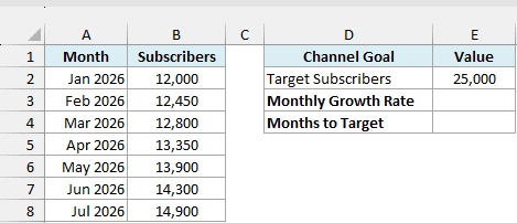
First, I need the monthly growth rate. Here is the formula that calculates it in cell E3:
=RRI(6,B2,B8)
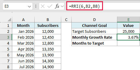
The RRI function returns the steady growth rate between a starting and an ending value. I’ve used 6 as the number of periods because seven month-end counts (January to July) have six months of growth between them.
So the channel has been growing at 3.67% a month. Now I can use this rate in PDURATION.
Here is the formula that gives the months needed:
=PDURATION(E3,B8,E2)
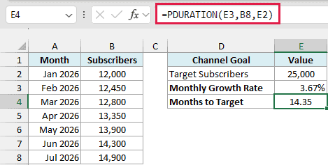
This formula uses the monthly rate from E3, the latest count of 14,900 in B8, and the target of 25,000 in E2. It returns 14.35, so at the current pace, the channel reaches 25,000 subscribers in a little over 14 months.
RRI and PDURATION work as a pair. RRI finds the rate when you know the number of periods, and PDURATION finds the number of periods when you know the rate.
If you add more months to the history, change the 6 to the new number of growth steps, and change B8 in both formulas to the new last cell. Otherwise, both formulas keep using the January to July data.
Example 7: When the Value Is Shrinking (PDURATION vs NPER)
Now let me show you a situation where PDURATION doesn’t work, which is when a value goes down instead of up.
Below are the details of a used car that loses 15% of its value every year (entered as -15% in B2), and I want to find how many years until it drops from $30,000 to a trade-in value of $12,000 in cell B7.
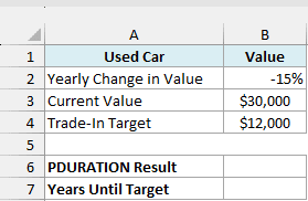
Here is what happens when I use PDURATION in cell B6:
=PDURATION(B2,B3,B4)
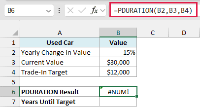
It returns the #NUM! error. This is because PDURATION only accepts a rate greater than zero, and the -15% in B2 is a negative rate.
And if you keep the rate positive and just put a target smaller than the starting value, you don’t get an error. Instead, PDURATION returns a negative number, which doesn’t make sense for this question.
To handle a shrinking value, use the NPER function. Here is the formula in cell B7:
=NPER(B2,0,-B3,B4)
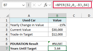
This returns 5.64, so the car reaches the $12,000 trade-in value in about 5.6 years.
In this formula, B2 is the -15% yearly change, 0 means there are no regular payments, -B3 is the current value, and B4 is the target value.
The minus sign in front of B3 is needed because NPER treats money going out and money coming in with opposite signs.
For a growing value with no regular payments, NPER gives the same answer as PDURATION. PDURATION is just simpler because you don’t need the 0 or the minus sign.
So this is how you can use the PDURATION function in Excel to find how long it takes for a value to reach a target.
Just make sure the rate matches the period you want the answer in. And switch to NPER when the value is shrinking or when you’re adding money regularly.
Other Excel Articles You May Also Like:
