

The OCT2DEC function in Excel converts an octal number into a regular decimal number. So 17 becomes 15, and 144 becomes 100.
Octal is a base-8 number system that uses only the digits 0 to 7. You won’t run into it every day, but it still shows up in Linux file permissions (755, 644) and some program output, and that’s when this function comes in handy.
One thing to know upfront. Like a few other older Excel functions, OCT2DEC won’t take a range of cells, so pointing it at a whole column returns a single #VALUE! error (Example 2 shows the fix).
Follow along with the example file
OCT2DEC Function Examples.xlsx
OCT2DEC Function Syntax
Here is the syntax of the OCT2DEC function:
=OCT2DEC(number)
- number is the octal number you want to convert. It can have at most 10 characters, and it’s the only argument.
You can point number to a cell, or type the octal value straight into the formula. Since octal values are made of digits only, you don’t need quotes, so =OCT2DEC(144) and =OCT2DEC("144") both return 100.
A 10-character octal number that starts with 4, 5, 6, or 7 is read as a negative number. I’ll show you how that works in Example 5.
The OCT2DEC function works in Microsoft 365 (Windows and Mac), Excel 2024, 2021, 2019, and 2016. The formulas in this tutorial that fill several cells at once need Microsoft 365, Excel 2024, or Excel 2021.
When to Use the OCT2DEC Function
Use this function when you need to:
- Convert a list of octal numbers into decimal numbers.
- Turn Linux file permission codes like 755 into their decimal values.
- Decode text that’s written as backslash octal codes.
- Read negative numbers stored as 10-digit octal values.
Let me show you a few practical examples of how to use OCT2DEC.
Example 1: Convert Octal to Decimal in Excel
Let’s start with a simple example.
Below is a list of octal numbers, and I want to convert each one into a decimal number in column B.
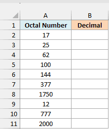
Here is the formula, entered in cell B2 and copied down to B11:
=OCT2DEC(A2)
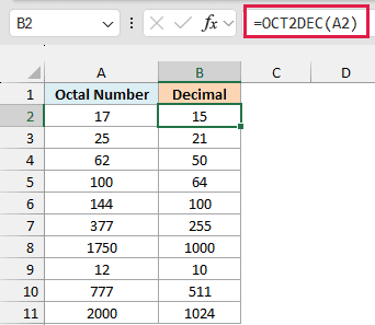
The formula converts each octal number in column A into its decimal value. For example, 17 becomes 15, 377 becomes 255, and 1750 becomes 1000.
Octal uses only the digits 0 to 7, and each position is worth 8 times the one to its right. So 144 is 1 x 64, plus 4 x 8, plus 4, which is 100.
The values in column A are regular numbers, and that’s fine. OCT2DEC reads the digits you see in the cell, so you don’t need to format the cells as Text before typing octal values.
If a value has a character that isn’t 0 to 7 (like an 8, a 9, a decimal point, a space, or a minus sign), or has more than 10 characters, OCT2DEC returns a #NUM! error. A blank cell returns 0.
I’ve used one formula per row here because it’s the simplest form, and it works in every Excel version. In the next example, I’ll show you how to convert the whole list with one formula.
Example 2: Convert a Whole List of Octal Values With One Formula
Now let’s do the same thing with a single formula.
Below is another list of octal numbers, and I want the decimal value of each one in column B using just one formula.
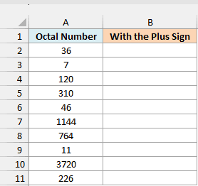
Here is the formula:
=OCT2DEC(+A2:A11)
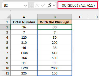
This converts all ten octal numbers at once, and the results spill down from B2 (Excel fills the cells below automatically). For example, 1144 becomes 612, and 3720 becomes 2000.
Notice the plus sign before A2:A11. Here is what you get if you leave it out, which I’ve entered in cell D2:
=OCT2DEC(A2:A11)
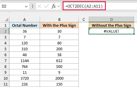
This time there’s just one #VALUE! error in D2, and nothing spills. OCT2DEC is one of the older functions that won’t take a range of cells as its input, even in Microsoft 365.
Adding the plus sign turns A2:A11 into a calculation, so Excel reads the values in those cells first. OCT2DEC then gets a list of values instead of a cell range, and it returns one result for each row.
You can read more about this trick in my article on Excel functions that won’t spill.
If you are using Excel 2019 or earlier, enter the below formula in cell B2 and then copy it down to B11:
=OCT2DEC(A2)
The same idea works for the other spilling formulas in this tutorial. In Excel 2019 or earlier, replace the range with its first cell (and drop the plus sign), then copy the formula down.
Example 3: Convert Linux File Permissions to Decimal
Here’s another practical scenario.
Below is a list of files with their Linux permission codes, and I want the decimal value of each code in column C.
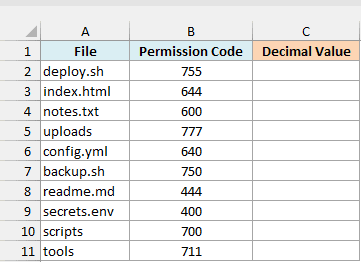
A permission code like 755 is an octal number.
Each digit sets the permissions for one group of users: the owner, the group, and everyone else. A digit adds up 4 for read, 2 for write, and 1 for run, so 7 (4+2+1) allows all three, and 5 (4+1) allows read and run.
So 755 means the owner can read, write, and run the file, while the group and everyone else can read and run it.
Some scripts and programs expect this setting as a plain decimal number instead of the octal code, and OCT2DEC gives you that number.
Here is the formula:
=OCT2DEC(+B2:B11)
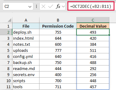
This converts every permission code into its decimal value, so 755 becomes 493, 644 becomes 420, and 777 becomes 511.
I’ve used the plus sign again because B2:B11 is a range of cells. Without it, you’d get the same single #VALUE! error you saw in Example 2.
Example 4: Decode Octal Character Codes Into Text
Now let’s look at something more interesting.
Below is a list of product names that were exported as octal character codes, and I want the readable product name in column B.
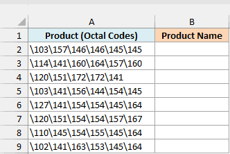
Each character here is written as a backslash followed by its 3-digit octal code. For example, \103 is the code for C, and \157 is the code for o.
You’ll see text written this way in some program logs and code.
Here is the formula in cell B2, copied down to B9:
=CONCAT(CHAR(OCT2DEC(TEXTSPLIT(A2,"\",,TRUE))))
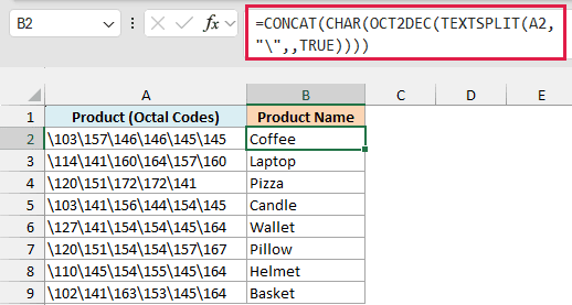
How this formula works:
TEXTSPLIT(A2,"\",,TRUE)uses the TEXTSPLIT function to split the text at every backslash. For Coffee, this gives 103, 157, 146, 146, 145, and 145.- The TRUE at the end tells the TEXTSPLIT function to skip empty pieces. The text starts with a backslash, so without it, the first piece would be empty and the formula would return
#VALUE!. - OCT2DEC converts each piece into a decimal number, so 103 becomes 67 and 157 becomes 111.
- The CHAR function returns the character for each number (67 is C and 111 is o), and the CONCAT function joins them back into one word.
You don’t need the plus sign here, because the TEXTSPLIT function already hands OCT2DEC a list of values instead of a cell range.
I’ve kept this as one formula per row because the TEXTSPLIT function splits one piece of text at a time.
If you point it at the whole range A2:A9, it returns only the first code from each row, so you’d get CLPCWPHB (the first letter of every product) in a single cell.
The TEXTSPLIT function is only available in Microsoft 365 and Excel 2024, so this formula won’t work in Excel 2021 or earlier.
Example 5: Convert Negative Octal Numbers (Two’s Complement)
Now let’s look at how OCT2DEC handles negative numbers.
Below is a list of 10-digit octal values (some positive and some negative), and I want their decimal values in column B.
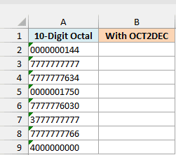
Here is the formula:
=OCT2DEC(+A2:A9)
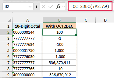
The values that start with 0 to 3 are positive, so they convert normally. For example, 0000000144 becomes 100, and 0000001750 becomes 1,000.
The ones that start with 4 to 7 are negative. OCT2DEC uses a system called two’s complement, where 7777777777 means -1, 7777777634 means -100, and 7777776030 means -1,000.
This only happens with 10-digit values. A shorter value is always positive, so 777 is 511 and 777777777 (nine digits) is 134,217,727.
The largest number OCT2DEC can return is 536,870,911 (3777777777), and the smallest is -536,870,912 (4000000000).
I’ve stored the values in column A as text so the leading zeros stay visible. OCT2DEC gives the same results if you type them as numbers, because the leading zeros don’t change the value.
Important: If your 10-digit values are IDs or sizes that are never meant to be negative, OCT2DEC gives you the wrong numbers for the ones starting with 4 to 7. Use the DECIMAL function instead, because it reads every value as a positive number.
Here is the DECIMAL function formula, which I’ve entered in cell D2:
=DECIMAL(A2:A9,8)
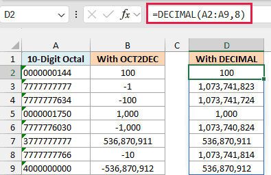
The 8 tells the DECIMAL function that the values are in base 8 (octal). The positive rows match column B, but the negative ones come back as large positive numbers, so 7777777777 becomes 1,073,741,823.
That gives you an easy way to see how two’s complement works. The number 1,073,741,824 is 8 to the power of 10, which is one more than the largest 10-digit octal value (7777777777).
Subtract 1,073,741,824 from the value the DECIMAL function returns for a negative row, and you get the OCT2DEC result. So 1,073,741,823 minus 1,073,741,824 is -1.
The DECIMAL function was added in Excel 2013, so it isn’t available in Excel 2010 or earlier.
Example 6: Convert Octal Numbers Longer Than 10 Digits
Now let’s look at what to do when your octal values are too long for OCT2DEC.
Below is a list of files with their sizes taken from a tar archive, and I want each size in bytes in column C.
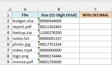
A tar archive is a common way to bundle files on Linux, and it stores the size of each file as an 11-digit octal number. OCT2DEC can’t read these, because it only takes 10 characters, but the DECIMAL function doesn’t have that limit.
Here is the formula in cell C2:
=DECIMAL(B2:B9,8)
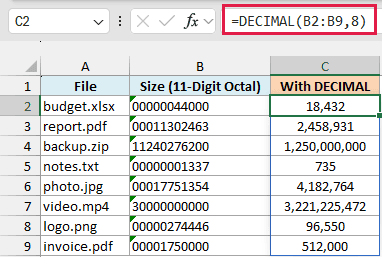
This converts every size into bytes, so 00000044000 becomes 18,432, and 30000000000 becomes 3,221,225,472. The DECIMAL function accepts a range directly, so you don’t need the plus sign here.
To show you what OCT2DEC does with these values, I’ve entered it in cell E2:
=OCT2DEC(+B2:B9)
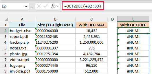
Every result is a #NUM! error, because each value has 11 characters. This happens even for small sizes like 00000001337, because the leading zeros still count as characters.
In this tutorial, I showed you how the OCT2DEC function works, how to convert a whole list with the plus-sign trick, and how to turn Linux permission codes into decimal values.
I also showed you how to decode octal character codes into text, how negative octal numbers work, and how to handle values longer than 10 digits.
If you need to go the other way, the DEC2OCT function converts decimal numbers back to octal. I hope you found this tutorial useful.
Other Excel Articles You May Also Like:
