

The DEC2OCT function converts a regular (decimal) number into octal, a number system that counts with only eight digits, 0 to 7. For example, =DEC2OCT(64) returns 100, because 100 in octal means 8 times 8, the same way 100 in decimal means 10 times 10.
You won’t need octal in everyday spreadsheets, but it shows up in computer work, like Linux file permissions and character codes.
This tutorial covers converting a whole column in one go, padding results with zeros, negative numbers, and what to do when a number is too big for DEC2OCT.
Follow along with the example file
DEC2OCT Function Examples.xlsx
DEC2OCT Function Syntax
Here is the syntax of the DEC2OCT function:
=DEC2OCT(number, [places])
- number – the decimal number you want to convert. It must be between -536,870,912 and 536,870,911, and it can be a number, a cell reference, or a number stored as text. If it has a decimal part, DEC2OCT drops it (Example 6 shows this).
- places – (optional) the number of characters you want in the result. DEC2OCT adds leading zeros to reach this length.
When you leave out places, DEC2OCT uses as few characters as it needs. So =DEC2OCT(20) returns 24, while =DEC2OCT(20,4) returns 0024.
If places is smaller than the result needs, you get a #NUM! error. For example, =DEC2OCT(100,2) returns #NUM! because 100 converts to 144, which needs three characters.
A places value of 0 or less also returns #NUM!, and text like “three” returns #VALUE!. If places has a decimal part, it’s cut down to a whole number, so 2.9 works like 2.
The DEC2OCT function works in Excel for Microsoft 365, Excel 2024, 2021, 2019, 2016, and Excel for Mac.
When to Use the DEC2OCT Function
Use this function when you need to:
- Convert regular decimal numbers into octal (base 8).
- Get octal codes of a fixed length, with leading zeros.
- Turn file mode numbers from Linux or Mac into permission codes like 644.
- Convert negative numbers into the 10-character octal form that computers use.
Let me show you a few practical examples of how to use the DEC2OCT function.
Example 1: Convert a List of Decimal Numbers to Octal
Let’s start with a simple example.
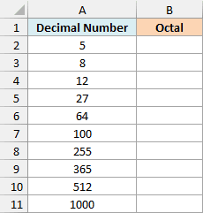
Below is a list of decimal numbers, and I want to convert each one to octal in column B.
Here is the formula:
=DEC2OCT(+A2:A11)
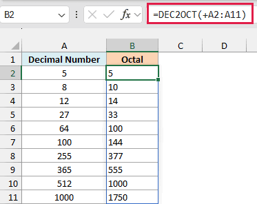
You enter this formula once in cell B2, and the results spill down to B11. DEC2OCT converts every number in A2:A11 to octal.
Important: Don’t skip the plus sign (+) before A2:A11. DEC2OCT can’t take a range reference directly, so =DEC2OCT(A2:A11) returns a single #VALUE! error instead of ten results.
The plus sign makes Excel read the values out of the range first and pass them to DEC2OCT as a list (an array), which it can work with. You’ll see the same plus sign in most examples below.
DEC2OCT isn’t the only function that behaves like this. Here’s a look at other Excel functions that won’t spill on a range, and how to fix them.
To see how the conversion works, remember that each place in an octal number is worth 8 times the place to its right (1, 8, 64, 512, and so on). So 100 is one 64, four 8s, and four 1s, which gives 144.
That’s also why 8 becomes 10, 64 becomes 100, and 512 becomes 1000. They are 8, 8 times 8, and 8 times 8 times 8, just like 10, 100, and 1000 in decimal.
Also notice that the results sit on the left of the cells. That’s because DEC2OCT returns text, not a number, even when the result looks like one.
If you are using Excel 2019 or earlier, enter the below formula in cell B2 and then copy it down the range:
=DEC2OCT(A2)
This version doesn’t need the plus sign, because each formula points to just one cell. The same copy-down approach works for the other examples in this article.
Example 2: Convert Characters to 3-Digit Octal Codes
Now let’s use the places argument.
Every character you type has a number code (A is 65, for example). Some programming languages and command-line tools write these codes as three octal digits, like \101 for A.
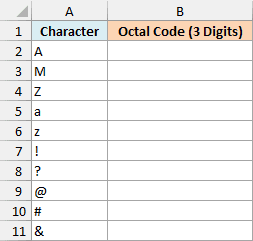
Below is a list of characters, and I want the code for each one as a 3-digit octal number in column B.
Here is the formula:
=DEC2OCT(CODE(A2:A11),3)
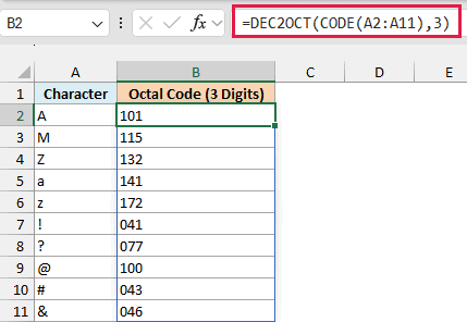
How this formula works:
- The CODE function returns the number code of each character. A gives 65, and ! gives 33.
- DEC2OCT then converts each code to octal, so 65 becomes 101.
- The 3 for places pads short results with leading zeros. The ! code converts to 41, so it comes back as 041.
Three characters is always enough here. The CODE function returns numbers up to 255, and 255 in octal is 377.
You don’t need the plus sign in this formula, because the CODE function already hands DEC2OCT a list of values rather than a range reference.
The same goes for any function that returns a list. For example, =DEC2OCT(SEQUENCE(64,1,0)) gives you a quick octal chart for 0 to 63.
If you want the backslash in front of each code, join it in with ="\"&DEC2OCT(CODE(A2:A11),3).
Example 3: Convert File Mode Numbers to Permission Codes
This one comes up if you work with files on Linux or Mac.
File permissions there are written as a 3-digit octal code like 644 or 755. But when you export a list of files with a script (Python’s os.stat, for example), you often get a single decimal number called the mode, like 33188.
The mode stores two things in one number: whether the item is a file or a folder, and its permissions.
Below is a list of files and folders with their decimal mode numbers, and I want the octal mode in column C and the 3-digit permission code in column D.
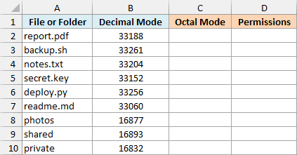
Here is the formula for the octal mode:
=DEC2OCT(+B2:B10)
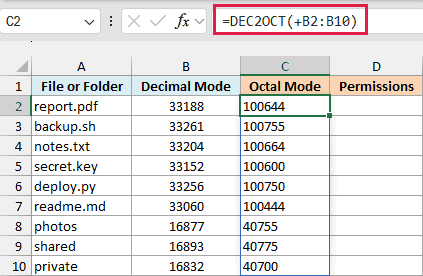
This converts every mode number to octal, so 33188 becomes 100644. The last three digits are the permissions (644).
The digits before them tell you what kind of item it is. 100 means a regular file and 40 means a folder, which is why the photos folder (16877) comes back as 40755.
Now here is the formula that pulls out the permission code:
=RIGHT(C2:C10,3)
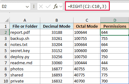
The RIGHT function takes the last three characters of each octal mode. The permissions are always the last three octal digits, so this works for files and folders alike.
Each of the three digits covers one group of people: the owner, the owner’s group, and everyone else.
Each digit adds up 4 for read, 2 for write, and 1 for execute, so 755 means the owner can do everything, while the others can read and run the file.
Example 4: Convert Negative Numbers With DEC2OCT
Now let’s look at negative numbers, which work a bit differently.
DEC2OCT shows a negative number as a 10-character octal number, using a system called two’s complement notation. It’s the same idea computers use to store negative whole numbers.
Below is a list of numbers, most of them negative, and I want their octal versions in column B, three characters long.
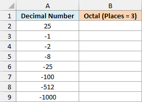
Here is the formula:
=DEC2OCT(+A2:A9,3)
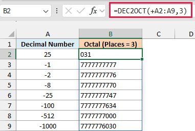
The positive number works just like in Example 2. 25 converts to 31, and places pads it to 031.
The negative ones come back as 10 characters that start with a run of 7s, even though I asked for three. -1 returns 7777777777, the largest 10-character octal number, and -2 is one less, 7777777776.
Behind the scenes, DEC2OCT adds the negative number to 1,073,741,824 (which is 10000000000 in octal) and converts the result. So -100 becomes 1,073,741,724, which is 7777777634 in octal.
In this 10-character form, any result that starts with 4, 5, 6, or 7 is a negative number (small negatives like these start with a run of 7s).
Trimming those leading digits would change the value, which is why DEC2OCT ignores places for negative numbers and always returns 10 characters.
To get the original number back, use the OCT2DEC function. For example, =OCT2DEC("7777777634") returns -100.
The smallest number DEC2OCT accepts is -536,870,912, which returns 4000000000. Anything lower returns a #NUM! error.
Example 5: Convert Numbers Larger Than 536,870,911
Now let’s push DEC2OCT past its limit.
Below is a list of numbers that get larger as you go down, and I want to try DEC2OCT in column B and then get the octal values with a method that works in column C.
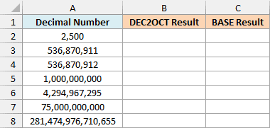
Here is the DEC2OCT formula:
=DEC2OCT(+A2:A8)
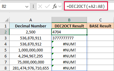
The first two numbers convert fine, but everything from 536,870,912 onward returns the #NUM! error.
DEC2OCT is limited to 10 octal characters, and the 10-character results that start with 4 to 7 are kept for negative numbers (as you saw in Example 4). So 536,870,911 (3777777777) is the largest positive number it can return.
Now here is the formula that works:
=BASE(A2:A8,8)
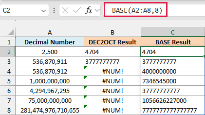
The BASE function converts a number into another number system, and the 8 tells it to use base 8, which is octal. So 1,000,000,000 becomes 7346545000.
BASE accepts a range directly, so this formula doesn’t need the plus sign. It works for numbers up to 9,007,199,254,740,991, and if you want leading zeros, its third argument sets the length (for example, =BASE(A2:A8,8,16)).
Important: The BASE function doesn’t accept negative numbers and returns #NUM! for them. For negative numbers, stick with DEC2OCT as shown in Example 4.
The BASE function is available in Excel 2013 and later versions.
Example 6: How DEC2OCT Handles Decimals, Text, and Empty Cells
Lastly, let’s look at what DEC2OCT does with inputs that aren’t plain whole numbers.
Below are some inputs that often cause surprises, with a note on what’s in each cell, and I want to see what DEC2OCT returns for each one in column C.
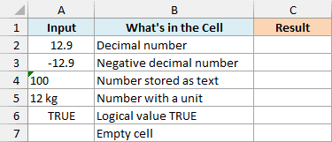
Here is the formula:
=DEC2OCT(+A2:A7)
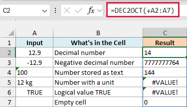
12.9 returns 14, which is 12 in octal. DEC2OCT drops the decimal part without rounding, and it does the same for negative numbers, so -12.9 is treated as -12 and returns 7777777764.
The 100 in cell A4 is stored as text, but DEC2OCT still converts it and returns 144. It reads text that looks like a number as that number.
12 kg returns the #VALUE! error because the unit makes it text that isn’t a number. The logical value TRUE returns #VALUE! as well.
Important: Two of these results look valid but may not be what you want. DEC2OCT cuts 12.9 down to 12 instead of rounding it to 13, and it treats the empty cell in A7 as 0 and returns 0.
If you want rounding, round the number first, for example with =DEC2OCT(ROUND(A2,0)), which returns 15 for 12.9. And make sure every input cell has a value, so a 0 in the results always means a real 0.
So these are a few examples of how to use the DEC2OCT function in Excel. Remember the plus sign when you convert a whole range, and switch to the BASE function for numbers above 536,870,911.
If you need to go the other way, the OCT2DEC function converts octal back to decimal. And for binary and hexadecimal, Excel has the DEC2BIN and DEC2HEX functions.
Other Excel Articles You May Also Like:
