

The HEX2DEC function in Excel converts a hexadecimal (hex) number into a regular decimal number. So FF becomes 255, and 1F becomes 31.
You’ll run into hex values in color codes, Unicode character codes, computer IDs, and data exported from apps and devices. When you need the actual number behind one of these codes, HEX2DEC gives it to you in one step.
There’s one catch, though. HEX2DEC is one of Excel’s older functions that won’t accept a range of cells, so pointing it at a whole column gives you a single #VALUE! error (Example 2 shows the fix).
Follow along with the example file
HEX2DEC Function Examples.xlsx
HEX2DEC Function Syntax
Here is the syntax of the HEX2DEC function:
=HEX2DEC(number)
- number is the hexadecimal number you want to convert. It can have at most 10 characters, and it’s the only argument.
You can point number to a cell, or type the hex value straight into the formula. When you type it in, put it in double quotes, like =HEX2DEC("1F"), because a hex value with letters isn’t something Excel can read as a number.
Upper and lower case letters give the same result, so =HEX2DEC("ff") and =HEX2DEC("FF") both return 255.
A 10-character hex number that starts with 8, 9, or a letter from A to F is read as a negative number. I’ll show you how that works in Example 7.
The HEX2DEC function works in Microsoft 365, Excel 2024, 2021, 2019, and 2016, and the Microsoft 365, 2024, and 2021 versions also work on Mac. The formulas in this tutorial that fill several cells at once need Microsoft 365, Excel 2024, or Excel 2021.
When to Use the HEX2DEC Function
Use this function when you need to:
- Convert a list of hex codes into decimal numbers.
- Clean up hex values written with a 0x in front and convert them.
- Get the red, green, and blue values from hex color codes.
- Show symbols from their Unicode hex codes.
- Turn hex timestamps from an app or log into real dates.
Let me show you a few practical examples of how to use HEX2DEC.
Example 1: Convert Hex to Decimal in Excel
Let’s start with a simple example.
Below is a list of hex numbers, and I want to convert each one into a decimal number in column B.
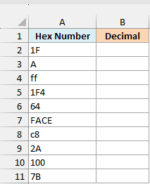
Here is the formula, entered in cell B2 and copied down to B11:
=HEX2DEC(A2)
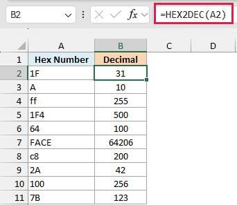
The formula converts each hex number in column A into its decimal value. For example, 1F becomes 31, 1F4 becomes 500, and FACE becomes 64206.
Hex uses the digits 0 to 9 and then the letters A to F for the values 10 to 15. Each position is worth 16 times the one to its right, so 1F is 1 x 16 plus 15, which is 31.
Notice that ff and c8 are in lowercase, and they still convert to 255 and 200. Also, the results are aligned to the right because HEX2DEC returns real numbers, so you can use them in other calculations.
If a value has a character that isn’t 0 to 9 or A to F (including a space or a minus sign), or has more than 10 characters, HEX2DEC returns a #NUM! error.
Important: If you type a hex value like 1E5 into a normal cell, Excel reads it as the number 1E+05 (100000), and HEX2DEC returns 1048576 instead of 485. Format the cells as Text before typing hex values, which is what I’ve done in column A.
I’ve used one formula per row here because it’s the simplest form, and it works in every Excel version. In the next example, I’ll show you how to convert the whole list with one formula.
Example 2: Convert a Whole List of Hex Values With One Formula
Now let’s do the same thing with a single formula.
Below is another list of hex numbers, and I want the decimal value of each one in column B using just one formula.
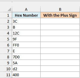
Here is the formula:
=HEX2DEC(+A2:A11)
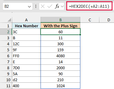
This converts all ten hex numbers at once, and the results spill down from B2 (Excel fills the cells below automatically). For example, 12C becomes 300, and 7D0 becomes 2000.
Notice the plus sign before A2:A11. Here is what you get if you leave it out, which I’ve entered in cell D2:
=HEX2DEC(A2:A11)
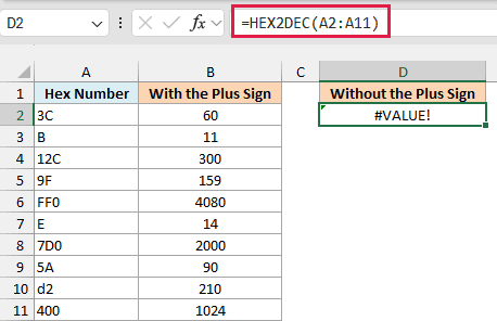
This time there’s just one #VALUE! error in D2, and nothing spills. HEX2DEC is one of the older functions (like the EOMONTH function) that won’t take a range of cells as its input, even in Microsoft 365.
Adding the plus sign turns A2:A11 into a calculation, so Excel reads the values in those cells first. HEX2DEC then gets a list of values instead of a cell range, and it returns one result for each row.
You can read more about this trick in my article on Excel functions that won’t spill.
If you are using Excel 2019 or earlier, enter the below formula in cell B2 and then copy it down to B11:
=HEX2DEC(A2)
The same idea works for the other spilling formulas in this tutorial. In Excel 2019 or earlier, replace the range with its first cell (and drop the plus sign), then copy the formula down.
Example 4 is the one exception, and I’ve given its older-version formula in that example.
Example 3: Convert Hex With a 0x Prefix to Decimal
Here’s another practical scenario.
Below is a list of hex values that start with 0x (the way many programs and code write hex), and I want their decimal values in column B.
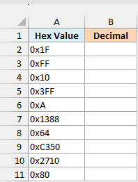
HEX2DEC can’t read these as they are, because x isn’t a hex digit, so every value would return #NUM!. The fix is to remove the 0x first.
Here is the formula:
=HEX2DEC(SUBSTITUTE(A2:A11,"0x",""))
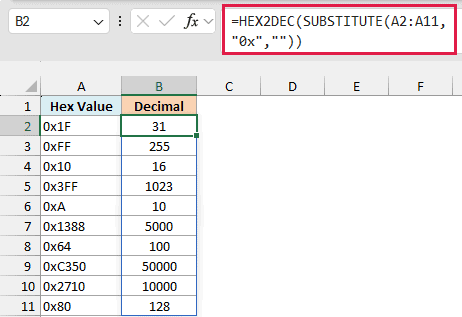
The SUBSTITUTE function replaces 0x with nothing in every value, so 0x1388 becomes 1388. HEX2DEC then converts what’s left, and 1388 becomes 5000.
You don’t need the plus sign here. The SUBSTITUTE function already hands HEX2DEC a list of values instead of a cell range, so the results spill down from B2.
The SUBSTITUTE function is case-sensitive, so a value written with a capital X (like 0X1F) keeps its prefix and still returns #NUM!. If your data has both, wrap the range in the UPPER function and replace “0X” instead.
Example 4: Get RGB Values From Hex Color Codes
Now let’s look at something more interesting.
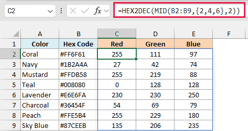
Below is a list of colors with their hex color codes, and I want the red, green, and blue values of each color in columns C, D, and E.
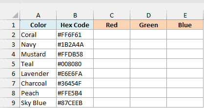
A hex color code is three 2-character hex numbers joined together, one each for red, green, and blue. Some tools ask for a color as these three separate numbers (each from 0 to 255) instead of a hex code.
Here is the formula in cell C2:
=HEX2DEC(MID(B2:B9,{2,4,6},2))
How this formula works:
MID(B2:B9,{2,4,6},2)uses the MID function to pull out 2 characters starting at positions 2, 4, and 6 of each code. Position 1 is the # sign, so it gets skipped.- For Coral’s #FF6F61, this gives FF, 6F, and 61. Because {2,4,6} is a row of three numbers, the MID function returns three columns for each of the eight codes.
- HEX2DEC converts all 24 pieces at once, so FF, 6F, and 61 become 255, 111, and 97.
One formula fills the whole C2:E9 block, and you don’t need the plus sign, because the MID function already hands HEX2DEC a list of values instead of a cell range.
If you are using Excel 2019 or earlier, enter the below formula in cell C2, copy it across to E2, and then copy it down to row 9:
=HEX2DEC(MID($B2,COLUMN(A1)*2,2))
Here, COLUMN(A1)*2 gives 2 in column C, and it changes to 4 and 6 as you copy the formula into columns D and E.
Example 5: Turn Unicode Hex Codes Into Symbols
Here’s one that’s handy when you need symbols in your sheet.
Below is a list of symbols with their Unicode codes (which are written in hex), and I want to show each symbol in column C.
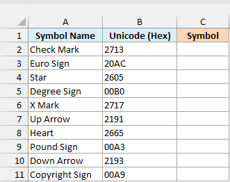
Here is the formula:
=UNICHAR(HEX2DEC(+B2:B11))
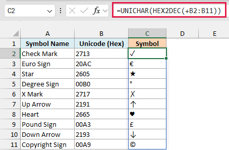
HEX2DEC converts each Unicode code into a decimal number. For example, 2713 becomes 10003, and 20AC becomes 8364.
The UNICHAR function then returns the character for that number, so 10003 gives you a check mark, and 8364 gives you the euro sign.
Unicode codes are always written in hex (often with a U+ in front, like U+2713), but the UNICHAR function only accepts a decimal number. That’s why you need HEX2DEC in between.
If your codes have the U+ in front, HEX2DEC returns #NUM! because U and + aren’t hex digits. Remove it first with the SUBSTITUTE function, the same way I removed 0x in Example 3.
The UNICHAR function was added in Excel 2013, so this example won’t work in Excel 2010 or earlier.
Example 6: Convert Hex Timestamps to Dates
Let’s step it up with a more advanced use case.
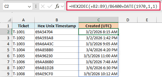
Below is a list of support tickets with the time each one was created, stored as a hex timestamp, and I want the actual date and time in column C.
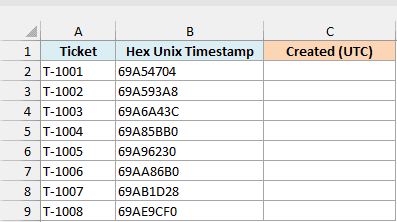
Some apps and databases record time as a Unix timestamp, which is the number of seconds since January 1, 1970 (in UTC). Sometimes that number is stored in hex, like the values in column B.
Here is the formula:
=HEX2DEC(+B2:B9)/86400+DATE(1970,1,1)
How this formula works:
HEX2DEC(+B2:B9)converts each hex timestamp into the number of seconds since January 1, 1970. For example, 69A54704 becomes 1772439300.- Dividing by 86400 (the number of seconds in a day) turns the seconds into days.
- Adding
DATE(1970,1,1)moves those days to the right spot in Excel’s date system, so 69A54704 becomes 3/2/2026 8:15 AM.
I’ve formatted column C to show the date and time. Without that format, you’d see a plain number like 46083.34 instead.
These results are in UTC. To show a local time, add or subtract the time difference as a fraction of a day, for example -5/24 for New York in winter.
Example 7: Convert Negative Hex Numbers (Two’s Complement)
Now let’s look at how HEX2DEC handles negative numbers.
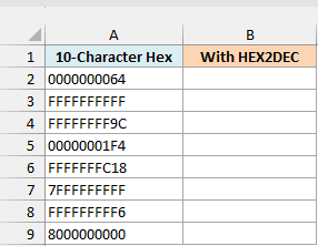
Below is a list of 10-character hex values (some positive and some negative), and I want their decimal values in column B.
Here is the formula:
=HEX2DEC(+A2:A9)
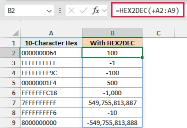
The values that start with 0 are positive, so they convert normally. For example, 0000000064 becomes 100, and 00000001F4 becomes 500.
The ones that start with 8 to F are negative. HEX2DEC uses a system called two’s complement, where FFFFFFFFFF means -1, FFFFFFFF9C means -100, and FFFFFFFC18 means -1,000.
This only happens with 10-character values. A shorter value is always positive, so FF is 255 and FFFFFFFFF (nine characters) is 68,719,476,735.
The largest number HEX2DEC can return is 549,755,813,887 (7FFFFFFFFF), and the smallest is -549,755,813,888 (8000000000).
If you want every value read as a positive number instead, use the DECIMAL function. Here is the formula, which I’ve entered in cell D2:
=DECIMAL(A2:A9,16)
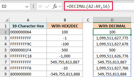
The 16 tells the DECIMAL function that the values are in base 16 (hex). The positive rows match column B, but the negative ones come back as large positive numbers, so FFFFFFFFFF becomes 1,099,511,627,775.
That gives you an easy way to see how two’s complement works. The number 1,099,511,627,776 is 16 to the power of 10, which is one more than the largest 10-character value (FFFFFFFFFF).
Subtract 1,099,511,627,776 from the value the DECIMAL function returns for a negative row, and you get the HEX2DEC result. So 1,099,511,627,775 minus 1,099,511,627,776 is -1.
The DECIMAL function was added in Excel 2013, so it isn’t available in Excel 2010 or earlier.
Important: Check where your hex values come from before using HEX2DEC on 10-character codes. If they are IDs or numbers that are never meant to be negative, HEX2DEC turns the ones starting with 8 to F into negative numbers, so use the DECIMAL function instead.
Example 8: Convert Hex Longer Than 10 Characters
Now let’s look at what to do when your hex values are too long for HEX2DEC.
Below is a list of devices with their MAC addresses (a 12-character hex ID every network device has), and I want each one as a decimal number in column C.
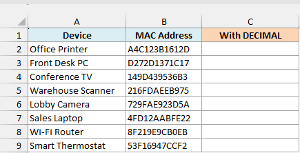
HEX2DEC can’t do this, because each MAC address has 12 characters and HEX2DEC only takes 10. The DECIMAL function doesn’t have that limit.
Here is the formula in cell C2:
=DECIMAL(B2:B9,16)
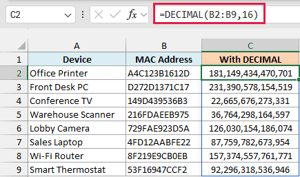
This converts every MAC address into a decimal number, so A4C123B1612D becomes 181,149,434,470,701. The DECIMAL function accepts a range directly, so you don’t need the plus sign here.
To show you what HEX2DEC does with these values, I’ve entered it in cell E2:
=HEX2DEC(+B2:B9)
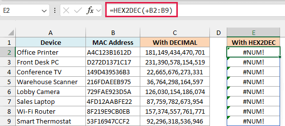
Every result is a #NUM! error, because each value has more than 10 characters.
MAC addresses are often written with colons or hyphens (like A4:C1:23:B1:61:2D). If yours are, remove those first with the SUBSTITUTE function, the same way I removed 0x in Example 3.
Important: Excel shows only 15 digits of a number, and every 12-character hex value fits in 15 digits, so these results are exact. With 13 or more characters, the result can need 16 digits or more, and Excel shows the extra digits as zeros.
In this tutorial, I showed you how the HEX2DEC function works, how to convert a whole list with the plus-sign trick, and how to deal with values that start with 0x.
I also showed you how to get RGB values from color codes, turn Unicode codes into symbols, convert hex timestamps into dates, and handle negative and extra-long hex values.
If you need to go the other way, the DEC2HEX function converts decimal numbers back to hex. I hope you found this tutorial useful.
Other Excel Articles You May Also Like:
