

The DEC2HEX function in Excel converts a decimal number (the everyday kind) into hexadecimal, which is base 16. So 255 becomes FF, and 4,095 becomes FFF.
You’ll run into hex in web color codes, network settings, and plenty of other tech stuff. DEC2HEX lets you do the conversion right in your sheet, and it can pad the results with leading zeros so they all have the same length.
Before you start, know that DEC2HEX won’t take a whole range of cells as its input. Point it at A2:A11 and you get a single #VALUE! error, but Example 1 shows a one-character fix.
Follow along with the example file
DEC2HEX Function Examples.xlsx
DEC2HEX Function Syntax
Here is the syntax of the DEC2HEX function:
=DEC2HEX(number, [places])
- number is the decimal number you want to convert. It has to be between -549,755,813,888 and 549,755,813,887. This argument is required.
- places is the number of characters you want in the result. This argument is optional.
When you leave out places, DEC2HEX returns as few characters as it needs. So =DEC2HEX(10) gives you A.
When you use places, DEC2HEX adds zeros in front of the result until it’s that many characters long. So =DEC2HEX(10,3) gives you 00A.
If number has decimals, DEC2HEX drops them before converting (it doesn’t round). So 255.9 is treated as 255, and you get FF.
Negative numbers work a little differently. They always come back as 10 characters, no matter what you use for places, and I’ll cover how that works in Example 5.
The DEC2HEX function works in all Excel versions, including Microsoft 365, Excel 2024, 2021, 2019, 2016, Mac, and the web. The single formulas in this tutorial that return a whole column of results need Microsoft 365, Excel 2024, or Excel 2021.
When to Use the DEC2HEX Function
Use this function when you need to:
- Convert a list of decimal numbers into hexadecimal.
- Create fixed-length hex codes with leading zeros, such as 0000C or 00FB5.
- Build hex color codes (like #FF6600) from RGB values.
- Convert an IP address into its 8-character hex form.
- Convert negative numbers into their hex form.
Let me show you how DEC2HEX works with a few practical examples.
Example 1: Convert a List of Decimal Numbers to Hex
Let’s start with a basic example.
Below is a list of numbers, and I want to convert each one into hexadecimal in column B.
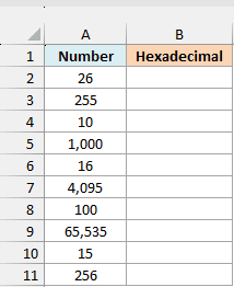
Here is the formula:
=DEC2HEX(+A2:A11)
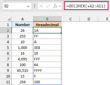
This one formula converts all ten numbers, and the results spill down from B2 (Excel fills the cells below on its own). For example, 26 becomes 1A, 1,000 becomes 3E8, and 65,535 becomes FFFF.
Hex counts in 16s instead of 10s. It uses the digits 0 to 9 and then the letters A to F for the values 10 to 15, which is why 10 becomes A, 15 becomes F, and 16 becomes 10.
Also notice that the results sit on the left side of the cells. That’s because DEC2HEX always returns text, even when the result looks like a regular number (like 64 or 100).
Now, about that plus sign before A2:A11. Here is the same formula without it, which I’ve entered in cell D2:
=DEC2HEX(A2:A11)
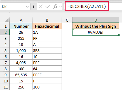
This time you get one #VALUE! error, and nothing spills. DEC2HEX is one of Excel’s older functions that won’t take a range of cells as its input, even in Microsoft 365.
The plus sign turns A2:A11 into a small calculation, so Excel hands DEC2HEX the values in those cells instead of the range itself. DEC2HEX then returns one result for each value.
You can read more about this trick in my article on Excel functions that won’t spill.
If you are using Excel 2019 or earlier, enter the below formula in cell B2 and then copy it down to B11:
=DEC2HEX(A2)
Example 2: Add Leading Zeros With the Places Argument
Here’s another practical scenario.
Below is a list of gym member numbers, and I want to turn each one into a short five-character hex code (to print on the key tags) in column B.
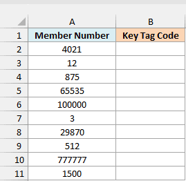
Here is the formula:
=DEC2HEX(+A2:A11,5)
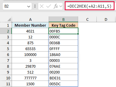
The 5 is the places argument. It tells DEC2HEX to make every result five characters long, so it adds zeros in front of the shorter ones: 12 becomes 0000C, 875 becomes 0036B, and 3 becomes 00003.
100000 and 777777 already need five characters (186A0 and BDE31), so they come back without any extra zeros. This way, every code on the list has the same length.
Important: If a number needs more characters than you ask for, DEC2HEX returns #NUM! instead of cutting the result short. For example, =DEC2HEX(1048576,5) gives you #NUM!, because its hex value (100000) needs six characters.
The places value itself has to be between 1 and 10. A 0, a negative number, or anything above 10 also returns #NUM!, and a decimal like 5.7 is cut down to 5.
You might think of using the TEXT function to add the zeros instead, but that only works on results made of digits. TEXT leaves a result like FF unchanged, so places is the way to go here.
Example 3: Convert RGB to Hex Color Codes in Excel
Now let’s look at something more fun.
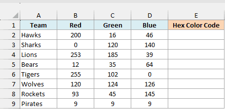
Below are the team colors for a local sports league, with the red, green, and blue (RGB) values of each color, and I want the hex color code for each team in column E.
Here is the formula:
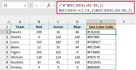
="#"&DEC2HEX(+B2:B9,2)&DEC2HEX(+C2:C9,2)&DEC2HEX(+D2:D9,2)
How this formula works:
DEC2HEX(+B2:B9,2)converts each red value into a two-character hex code, so 200 becomes C8. The other two DEC2HEX parts do the same for the green and blue values.- The & operator joins the three codes together, with a # in front. So the Hawks’ 200, 16, and 46 become C8, 10, and 2E, which gives you #C8102E.
Every hex color code needs exactly two characters for each color, which is why places is set to 2. The Sharks have a red value of 0, and places turns it into 00, giving you #00788C.
Without places, that 0 would come back as just 0, and you’d get #0788C, which isn’t a valid color code. The same goes for the Pirates, whose 9s need to become 09.
Pro Tip: Some style guides and CSS files write hex colors in lowercase (like #c8102e). To get that, wrap the whole formula in the LOWER function.
You can paste these codes into a website builder or any design tool that takes hex colors to get the exact same shades.
Example 4: Convert an IP Address to Hex
Some network tools and boot setups write an IP address as one hex value (like C0A8010A instead of 192.168.1.10), and DEC2HEX makes that conversion easy.
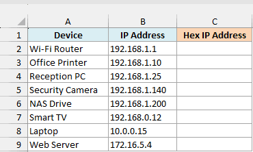
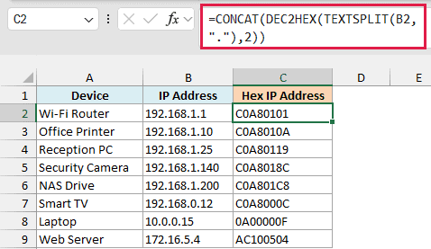
Below is a list of devices with their IP addresses, and I want each IP address written as one 8-character hex value in column C.
Here is the formula, entered in cell C2 and copied down to C9:
=CONCAT(DEC2HEX(TEXTSPLIT(B2,"."),2))
How this formula works:
TEXTSPLIT(B2,".")splits the IP address at each dot, so 192.168.1.1 (the Wi-Fi Router) becomes four separate values: 192, 168, 1, and 1.DEC2HEX(...,2)converts each of those four values into a two-character hex code, which gives you C0, A8, 01, and 01.CONCATjoins the four codes into one value, C0A80101.
Each part of an IP address is a number from 0 to 255, so it always fits in two hex characters.
The 2 (places) makes sure the small parts keep their leading zero. Without it, 192.168.1.1 would come out as C0A811 instead of C0A80101.
Places also catches typos. A part above 255 (like 300) needs three characters, so DEC2HEX returns #NUM! instead of giving you a wrong hex value.
Notice that there’s no plus sign this time. TEXTSPLIT already returns a list of values (not a range of cells), and DEC2HEX has no problem taking that.
I’ve used one formula per row here instead of a single formula for the whole column. If you point TEXTSPLIT at B2:B9, it returns only the first part of each IP address (192 for the first six rows, then 10 and 172).
CONCAT then joins those into one wrong value, C0C0C0C0C0C00AAC, instead of giving you a hex code for each row.
The TEXTSPLIT function is available only in Microsoft 365 and Excel 2024.
If you are using Excel 2021 or earlier (which don’t have TEXTSPLIT), first split the IP addresses into columns E to H. Use Text to Columns with the dot as the delimiter and E2 as the destination.
Then enter the below formula in cell C2 and copy it down to C9:
=DEC2HEX(E2,2)&DEC2HEX(F2,2)&DEC2HEX(G2,2)&DEC2HEX(H2,2)
Example 5: Convert Negative Numbers to Hex
Let’s step it up with a trickier case.
Below is a list of positive and negative numbers, and I want their hex values in column B, with the positive ones padded to four characters.
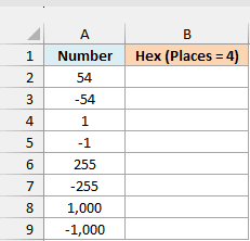
Here is the formula:
=DEC2HEX(+A2:A9,4)
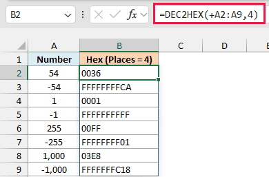
The positive numbers convert as usual and get padded to four characters, so 54 becomes 0036 and 1,000 becomes 03E8.
The negative numbers come back as 10-character values that start with F. For example, -54 becomes FFFFFFFFCA, and -1 becomes FFFFFFFFFF.
This is called two’s complement, which is the usual way computers store negative numbers. DEC2HEX works with 10 hex characters, and it writes a negative number by counting down from the largest 10-character value, so -1 is FFFFFFFFFF and -2 would be FFFFFFFFFE.
You’ll also notice that every negative result is 10 characters long, even though I asked for 4. That’s because DEC2HEX ignores the places argument for negative numbers and always returns all 10 characters.
If you ever need to go back the other way, the HEX2DEC function reads these 10-character values as negative numbers, so it turns FFFFFFFFCA back into -54.
Example 6: Convert Large Numbers to Hex (Beyond the DEC2HEX Limit)
Now let’s look at what to do when your numbers are too big for DEC2HEX.
Below is a list of storage devices with their capacity in bytes, and I want the hex value of each capacity in column C.
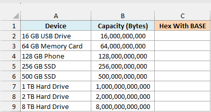
DEC2HEX only goes up to 549,755,813,887 (7FFFFFFFFF in hex), and the last three capacities in this list are bigger than that. So for this one, I’ll use the BASE function, which can convert a number into any base you want.
Here is the formula in cell C2:
=BASE(B2:B9,16)
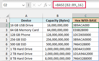
The 16 tells BASE to convert each number into base 16, which is hexadecimal. So 1,000,000,000,000 (the 1 TB drive) becomes E8D4A51000.
Unlike DEC2HEX, BASE accepts a range directly, so you don’t need the plus sign here.
To compare, here is DEC2HEX on the same list, which I’ve entered in cell E2:
=DEC2HEX(+B2:B9)
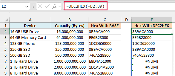
The first five results match the BASE results exactly. The last three return #NUM!, because those capacities are above the DEC2HEX limit.
Important: BASE can’t convert negative numbers (it returns #NUM!), and it only works for numbers below 2^53 (about 9 quadrillion). So for negative numbers, stick with DEC2HEX.
The BASE function was added in Excel 2013. If you are using Excel 2013, 2016, or 2019, enter the below formula in cell C2 and then copy it down to C9:
=BASE(B2,16)
So that’s how the DEC2HEX function works. You can use it to convert a single number or a whole list (with the plus-sign trick), and to pad the results with leading zeros using places.
I also showed you how to build hex color codes and hex IP addresses, what DEC2HEX does with negative numbers, and when to switch to BASE for really large numbers. I hope you found this tutorial useful.
Other Excel Articles You May Also Like:
