

If you want to break a piece of delimited text into separate pieces, like splitting a code at each pipe or a list at each comma, the TEXTSPLIT function is what you’re looking for.
You give it the text and the character to split on, and it does the rest.
TEXTSPLIT is a dynamic array function. It spills its results across the columns to the right, down the rows below, or both at once.
In this article, I’ll show you how to use TEXTSPLIT with 12 practical examples, from a simple split into columns to splitting a whole column of cells at once.
Follow along with the example file
TEXTSPLIT Function Examples.xlsx
TEXTSPLIT Function Syntax
Here is the syntax of the TEXTSPLIT function:
=TEXTSPLIT(text,col_delimiter,[row_delimiter],[ignore_empty],[match_mode],[pad_with])
- text – the text you want to split, or a cell that holds it.
- col_delimiter – the character or text that splits the result across columns.
- row_delimiter – optional. The character or text that splits the result down rows.
- ignore_empty – optional. Set it to TRUE to skip the empty pieces that two delimiters in a row create. It defaults to FALSE.
- match_mode – optional. Use 1 to match the delimiter without caring about letter case. It defaults to 0, which is case-sensitive.
- pad_with – optional. The value that fills missing cells when rows come out uneven. It defaults to the #N/A error.
You need at least one delimiter. Give TEXTSPLIT only a col_delimiter and the pieces go across columns.
Leave col_delimiter empty and give a row_delimiter, and the pieces go down rows. Give it both, and you get a full grid with rows and columns.
If the delimiter isn’t in the text at all, TEXTSPLIT simply returns the whole text in one cell.
TEXTSPLIT needs a real separator to split on. An empty delimiter (“”) returns #VALUE!, and it can’t tell where letters end and digits begin.
For that job, see how to separate text and numbers in Excel.
It also always returns text. Even “2010” comes back as text, which matters when you want to do math with the pieces (Example 8 shows the fix).
Important: TEXTSPLIT works in Excel for Microsoft 365, Excel for the web, and Excel 2024. In Excel 2021, 2019, or 2016, you’ll get a #NAME? error.
If you’re using an older version of Excel that doesn’t have TEXTSPLIT, you can get the same result with a combination of LEFT, MID, and FIND formulas.
Alternatively, you can use Text to Columns, which splits the data easily. Just remember that it gives you static results, so it won’t update if your original data changes.
If your Excel isn’t in English, the function has a translated name, but it works exactly the same way:
| Excel language | TEXTSPLIT is called |
|---|---|
| German | TEXTTEILEN |
| French | FRACTIONNER.TEXTE |
| Spanish | DIVIDIRTEXTO |
| Portuguese (Brazil) | DIVIDIRTEXTO |
| Italian | DIVIDI.TESTO |
| Dutch | TEKST.SPLITSEN |
When to Use the TEXTSPLIT Formula to Split Text in Excel
Use this function when you need to:
- Turn a delimited code, import, or pasted record into separate columns with one formula that updates when the source changes.
- Split a list down into rows without running Text to Columns and then transposing the result.
- Turn a block of text with line breaks into a proper table.
- Clean up messy separators by splitting on several delimiters, skipping empty pieces, or ignoring letter case.
- Feed the split pieces straight into other functions like SUM, SORT, UNIQUE, INDEX, or COUNTA.
Let me show you a few practical examples of how this works.
Example 1: Split a Cell into Columns (by Delimiter)
Let’s start with a simple case: splitting one cell across columns.
Below is the dataset. Cell A2 holds the movie record Inception|2010|Sci-Fi|148, with the movie name, release year, genre, and runtime in minutes joined by pipe characters.
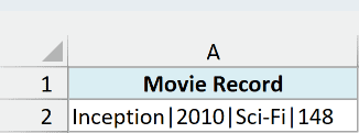
I want each field in its own column, starting in C2.
Here is the formula:
=TEXTSPLIT(A2,"|")

TEXTSPLIT looks through the text in A2, cuts it at every pipe, and drops each piece into the next cell to the right.
You type the formula once in C2, and the four values spill across C2:F2 on their own.
Because it’s a live formula, changing the record in A2 updates the split instantly. That’s the big difference from a one-time Text to Columns.
Notice that 2010 and 148 sit on the left side of their cells. That’s Excel telling you they came back as text, not numbers.
Pro Tip: You enter TEXTSPLIT once, in the top-left cell of the result, and keep the cells it spills into empty. There’s no need to drag it or press Ctrl + Shift + Enter.
Important: If you see a #SPILL! error, something is in the way. Clear any cells in the spill range, or move the formula out of an Excel Table.
Example 2: Split a Delimited List Down a Column
Here’s another common scenario, where you want the pieces stacked down a column instead of across.
Below is the dataset. Cell A2 contains a weekend to-do list, Buy groceries;Pay electricity bill;Call the dentist;Water the plants, with each task separated by a semicolon.

I want each task on its own row, starting in C2.
Here is the formula:
=TEXTSPLIT(A2,,";")
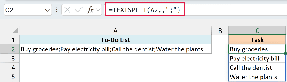
Notice the two commas after A2. The first spot is col_delimiter, and leaving it empty tells TEXTSPLIT not to split across columns.
The semicolon then goes in the row_delimiter spot, so the four tasks spill down C2:C5 instead of across.
Pro Tip: For more ways to handle this, including Text to Columns and a VBA option, see my guide on how to split text into rows in Excel.
Example 3: Split Text by Multiple Delimiters
Now let’s look at something messier, where the text uses more than one separator.
Below is the dataset. Cell A2 holds Yoga,,Zumba / Pilates;Spin, a list of fitness classes that mixes commas, a slash, and a semicolon.
The two commas in a row also leave an empty piece between them.
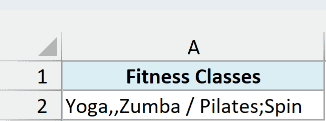
I want each class in its own column, without a blank cell for that empty piece.
Here is the formula:
=TEXTSPLIT(A2,{","," / ",";"},,TRUE)
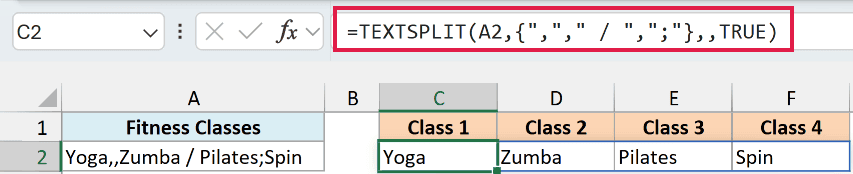
Here is how this formula works:
- The array constant {“,”,” / “,”;”} tells TEXTSPLIT to treat all three separators as delimiters. It splits wherever it finds any of them.
- The row_delimiter spot is left empty, so everything spills across columns.
- The final TRUE is the ignore_empty argument. It drops the empty piece from the double comma, so you get Yoga, Zumba, Pilates, and Spin with no gap.
Important: ignore_empty is FALSE by default, so two delimiters in a row leave a blank cell. The same goes for a delimiter at the very start or end of the text.
Also note that ” / ” includes the spaces around the slash. A delimiter can be more than one character, and TEXTSPLIT matches it exactly.
When your pieces come out with stray spaces because the spacing is inconsistent, wrap the whole TEXTSPLIT formula in TRIM.
Pro Tip: Delimiters are plain text, so wildcards like * and ? don’t work. And when one delimiter is part of another, like “,” and “, “, TEXTSPLIT uses the longer match.
Example 4: Split Text with Line Breaks into Rows and Columns
Let’s step it up with a two-dimensional split, where the result spills across and down at the same time.
Below is the dataset. Cell A2 holds three order records like ORD-101|Farah|Shipped.
The fields in each record are joined by pipes, and a line break separates one record from the next.
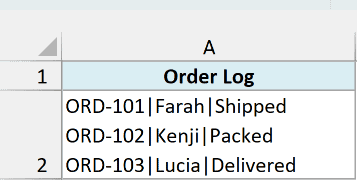
I want to turn that block of text into a table with the order ID, customer, and status in separate columns.
Here is the formula:
=TEXTSPLIT(A2,"|",CHAR(10))
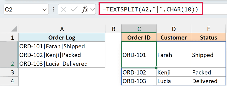
The pipe goes in the col_delimiter spot to break each record into columns.
CHAR(10) is the line break character. Putting it in the row_delimiter spot starts a new row at every line break, so you get a tidy grid in C2:E4.
A line break inside a cell comes from pressing Alt + Enter. If you want the details, here’s how to insert a line break in Excel.
Text imported from other programs can end each line with CHAR(13)&CHAR(10). Use that pair as the row_delimiter so no hidden character is left behind.
Example 5: Split Text Using a Case-Insensitive Delimiter
This next one uses the match_mode argument, which comes in handy when the word you split on shows up in different cases.
Below is the dataset. Cell A2 holds Delhi VIA Mumbai via Singapore, a travel route where the separator word appears once in capitals and once in lowercase.
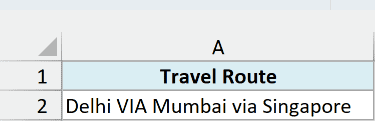
I want the three cities back as separate stops, even though the separators don’t match in case.
Here is the formula:
=TEXTSPLIT(A2," via ",,,1)
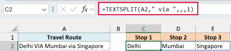
The delimiter here is ” via ” with a space on each side, so the spaces are removed along with the word.
The 1 in the fifth spot is match_mode. It tells TEXTSPLIT to ignore letter case, so it splits on both “VIA” and “via”.
Without that 1, TEXTSPLIT would be case-sensitive and only split on the lowercase “via”, leaving “Delhi VIA Mumbai” in one cell.
Example 6: Split and Pad Uneven Records (pad_with)
Here’s a scenario where the records don’t all have the same number of fields, which is exactly what the pad_with argument is for.
Below is the dataset. Cell A2 holds Pancakes,Breakfast,20;Caesar Salad,Lunch;Lasagna,Dinner,75.
There are three recipes separated by semicolons, and the middle one is missing its prep time.

I want a clean table, with the missing prep time showing “Not supplied” instead of an error.
Here is the formula:
=TEXTSPLIT(A2,",",";",FALSE,0,"Not supplied")
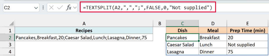
Here is how this formula works:
- The comma is the col_delimiter and the semicolon is the row_delimiter, so each recipe becomes a row split into columns.
- The Caesar Salad record only has two fields, so its third cell has nothing to show.
- The last argument, “Not supplied”, is pad_with. It fills that empty cell, giving you a neat three-by-three table with no error.
Important: Without pad_with, the missing cell shows #N/A. Set pad_with directly instead of wrapping the formula in IFNA, since the padding is already built into TEXTSPLIT.
I’ve typed FALSE and 0 here so you can see where each argument sits. They’re the defaults, so =TEXTSPLIT(A2,”,”,”;”,,,”Not supplied”) gives the same result.
Example 7: Get the First, Nth, or Last Value After Splitting
Quite often you don’t need every piece, just one of them. You can wrap TEXTSPLIT in another function to pick it out.
Below is the dataset. Cell A2 holds the address 742 Maple Avenue, Chicago, IL 60614, USA, with each part separated by a comma and a space.
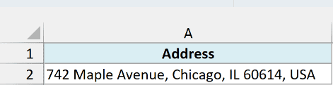
I want the city (the second item) in B4 and the country (the last item) in B5.
Here is the formula for the city:
=INDEX(TEXTSPLIT(A2,", "),2)
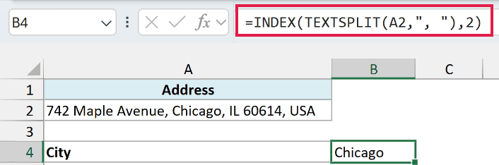
TEXTSPLIT splits the address into four pieces, and INDEX picks the second one, which is Chicago.
Change the 2 to 1 and you get the first item. Change it to 3 and you get the third.
And here is the formula for the country:
=TAKE(TEXTSPLIT(A2,", "),,-1)
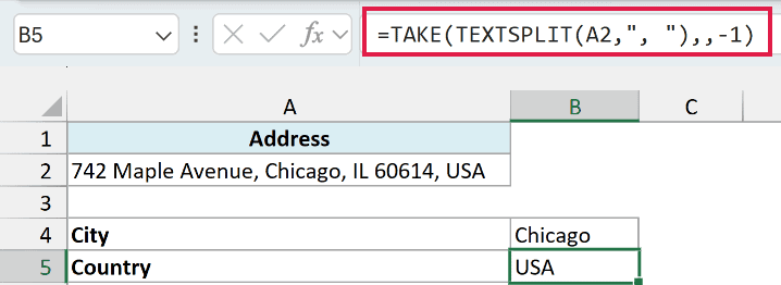
TAKE with -1 in its columns argument grabs the last column of the split result, which is USA.
This works no matter how many pieces the text has. And if you change -1 to -2, you get the last two items.
If the text you’re splitting is a full name, I have a separate guide on how to separate first and last name in Excel.
Pro Tip: If you only ever need the last item, =TEXTAFTER(A2,”, “,-1) is shorter. The -1 tells TEXTAFTER to return the text after the last delimiter.
Example 8: Sum Comma-Separated Numbers in a Cell
This one is easy to miss, because TEXTSPLIT always returns text, even when the pieces look like numbers.
Below is the dataset. Cell A2 holds a week of daily step counts, 8200,10450,7600,12300,9100,6800,11050, separated by commas.
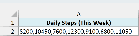
I want the total number of steps for the week.
Let me first show you what happens with a plain SUM:
=SUM(TEXTSPLIT(A2,","))
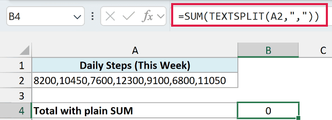
This returns 0. TEXTSPLIT hands SUM seven pieces of text, and SUM ignores text in an array, so there’s nothing left to add.
Here is the formula that fixes it:
=SUM(--TEXTSPLIT(A2,","))
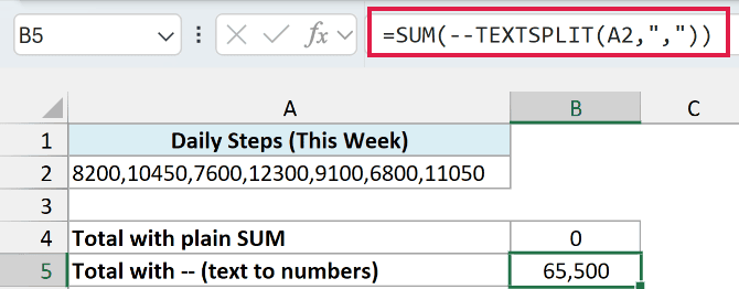
This gives us 65,500.
The double minus (–) in front of TEXTSPLIT converts each text piece into a real number. The first minus makes it negative, and the second flips it back.
Important: A split result that looks like a number is still text. Convert it with — or VALUE before you use it in SUM, AVERAGE, or a comparison.
Example 9: Use TEXTSPLIT on Multiple Cells (a Range)
So far every example split one cell. But what if you have a whole column of cells to split?
Below is the dataset. Cells A2:A7 each hold the toppings for one pizza order, like Cheese,Mushroom,Olive. Some orders have one topping and some have four.
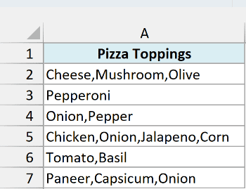
I want each order on its own row, with its toppings spread across the columns.
The obvious thing to try is giving TEXTSPLIT the whole range:
=TEXTSPLIT(A2:A7,",")
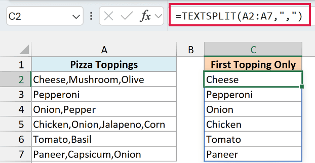
This doesn’t work the way you’d hope. You only get the first topping of each order in C2:C7.
That’s because each cell would split into its own row of results. A formula can’t return a list of lists, so Excel keeps just the first piece of each.
This limitation is often called the array of arrays problem.
Wrapping TEXTSPLIT in BYROW or MAP runs into the same wall and returns a #CALC! error. But there are two good ways around it.
The first is to join all the cells into one piece of text, then split that text in both directions:
=TEXTSPLIT(TEXTJOIN(";",FALSE,A2:A7),",",";",,,"")
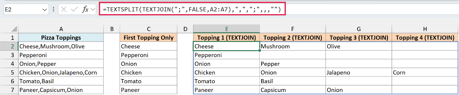
Here is how this formula works:
- TEXTJOIN joins the six cells into one long string, with a semicolon between each order.
- TEXTSPLIT then splits that string on commas across columns and on semicolons down rows, so each order becomes one row.
- Orders with fewer toppings leave gaps, and the “” at the end (pad_with) fills them with blanks instead of #N/A.
- FALSE in TEXTJOIN keeps empty cells, so a blank order still gets its own row and the results stay lined up with column A.
Important: TEXTJOIN can’t create text longer than 32,767 characters. On a very large list, this formula returns an error, so use the REDUCE version below instead.
The second way splits one cell at a time and stacks the results. It’s longer, but it avoids TEXTJOIN’s limit on the combined text:
=IFNA(DROP(REDUCE("",A2:A7,LAMBDA(acc,row,VSTACK(acc,TEXTSPLIT(row,",")))),1),"")
Worksheet and memory limits still apply, and repeated stacking can slow larger lists.
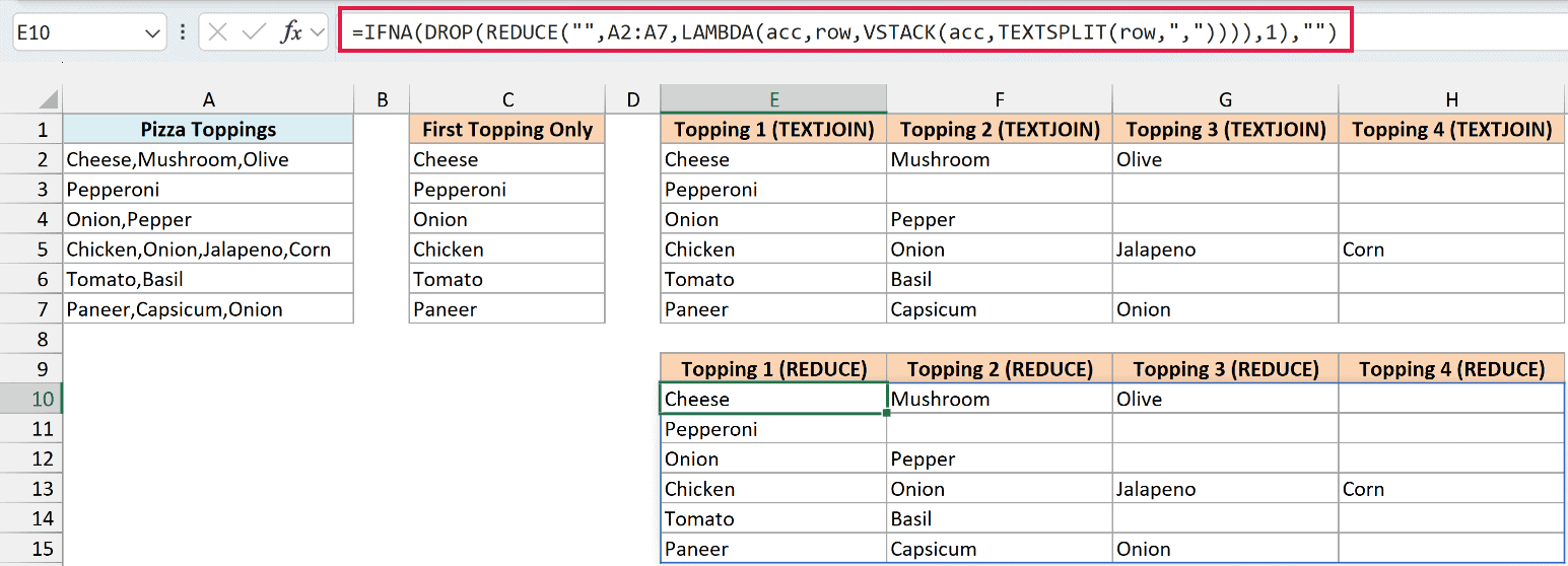
Here is how this formula works:
- REDUCE goes through A2:A7 one cell at a time, starting with an empty value (“”).
- For each cell, TEXTSPLIT splits the toppings, and VSTACK adds that row under everything built so far.
- DROP removes the empty starting row, and IFNA replaces the #N/A that VSTACK uses to pad shorter rows with blanks.
Both formulas give the same table. The TEXTJOIN version is shorter and faster, so use it for everyday lists.
Keep the REDUCE version for lists that are too big for TEXTJOIN.
If you’re splitting thousands of rows as part of a regular data cleanup, the Split Column option in Power Query is also worth a look.
Microsoft started testing nested arrays in the Beta Channel in September 2026. They let TEXTSPLIT return full results for a range, but for now, use the formulas above.
Example 10: Split Comma-Separated Values into Rows and Keep the Label
A close cousin of the last example is when each row has an ID plus a list, and you want one row per list item with the ID repeated.
Below is the dataset. Column A has four trip names and column B lists the cities in each trip, separated by a comma and a space, like Paris, Rome, Vienna.
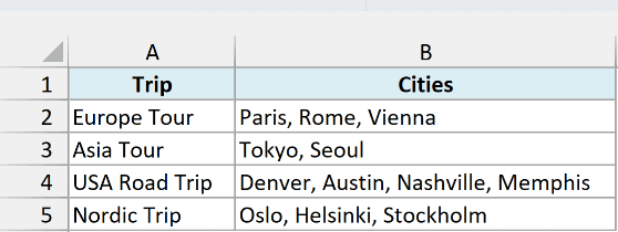
I want a two-column list in D2, with one city per row and its trip name next to it.
Here is the formula:
=LET(c,TEXTSPLIT(TEXTJOIN(";",FALSE,B2:B5),", ",";"),HSTACK(TOCOL(IF(ISNA(c),c,A2:A5),2),TOCOL(c,2)))
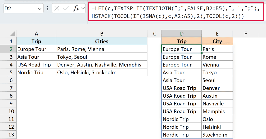
Here is how this formula works:
- TEXTJOIN joins the four city lists with a semicolon between trips. TEXTSPLIT then turns that into a grid, with one row per trip and one city per column.
- Shorter trips leave #N/A in their empty cells. LET stores this grid as c, so the formula can reuse it.
- IF(ISNA(c),c,A2:A5) builds a matching grid that has the trip name wherever there’s a city, and #N/A wherever there isn’t.
- TOCOL reads each grid row by row into a single column, and the 2 tells it to skip the #N/A cells. HSTACK then puts the trip column and the city column side by side.
Since both grids have their #N/A cells in exactly the same spots, the trip names and cities stay perfectly lined up.
Important: This formula also uses TEXTJOIN, so the same 32,767-character limit applies. For a very large table, build it row by row with REDUCE, as in Example 9.
Example 11: Combine Items from Multiple Cells into a Sorted Unique List
Let’s look at a more advanced use that pulls a few functions together.
Below is the dataset. Cells A2:A6 each hold a pipe-delimited grocery list, and some items like Milk and Eggs show up in more than one list.
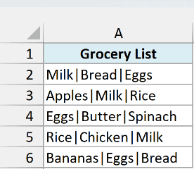
I want one clean list of every item in C2, sorted alphabetically, with the duplicates removed.
Here is the formula:
=SORT(UNIQUE(TEXTSPLIT(TEXTJOIN("|",TRUE,A2:A6),,"|")))
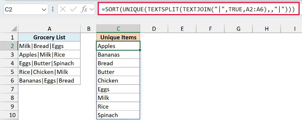
Here is how this formula works:
- TEXTJOIN stitches all five cells into one long string. It uses a pipe between cells too, so every item ends up separated the same way.
- TEXTSPLIT splits that string on the pipe into rows, using the empty col_delimiter from Example 2.
- UNIQUE removes the repeated items, and SORT puts the nine items that are left in alphabetical order.
TEXTSPLIT works on one text string at a time, so TEXTJOIN is what lets you fold a whole range into that single string first.
Here TRUE in TEXTJOIN skips empty cells, which is what you want, since a blank would otherwise show up as an empty item in the list.
The same 32,767-character TEXTJOIN limit from Example 9 applies here too.
Example 12: Count the Number of Items in Each Cell
Let’s finish with a simple question you’ll run into all the time: how many items are in each cell?
Below is the dataset. Column A has order numbers from a coffee shop, and column B lists the items in each order, separated by a comma and a space. Order A-104 was left empty.
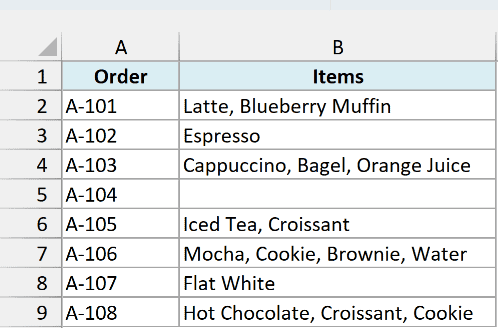
I want the number of items in each order in column C.
Here is the formula:
=BYROW(B2:B9,LAMBDA(items,IF(items="",0,COUNTA(TEXTSPLIT(items,", ",,TRUE)))))
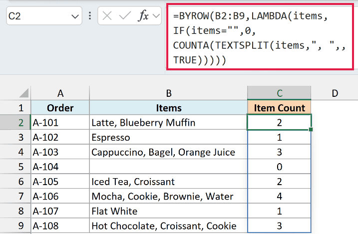
Here is how this formula works:
- BYROW goes through B2:B9 one cell at a time and passes each one to the LAMBDA as items.
- TEXTSPLIT splits the items, and COUNTA counts the pieces. TRUE skips empty pieces, so a stray extra comma doesn’t inflate the count.
- The IF returns 0 for an empty cell, which is why order A-104 shows 0.
The delimiter here is a comma and a space, but the method works the same with any delimiter. If your items are separated by a pipe or a hyphen, just change ", " in the formula to "|" or "-".
This time BYROW works fine, unlike in Example 9. That’s because each row returns just one number, not a whole list of pieces.
Important: TEXTSPLIT returns #VALUE! when the text is empty. COUNTA would count that error as 1, so keep the IF check for blank cells.
So these are 12 practical ways to use TEXTSPLIT in Excel, from a simple split into columns to splitting a whole column of cells at once.
Once you know which delimiter goes in which spot, and when to reach for ignore_empty, match_mode, and pad_with, you’ll find yourself using it all the time.
I hope you found this tutorial helpful.
Other Excel Articles You May Also Like:
