Excel REDUCE Function

REDUCE function is one of the hardest functions in Excel, and in this article, I will simplify it for you with lots of examples.

Reduce function is available in Excel for Microsoft 365, Excel for Microsoft 365 for Mac, and Excel for the web.

Click here to download the example file

What does the Reduce Function do?

The REDUCE function is a lambda helper function that processes each value in an array or range, one at a time, and accumulates them into a single final result.

Reduce Function Syntax

=REDUCE([initial_value], array, lambda(accumulator, value, body))

where:

• [initial_value] – This is your starting point. Think of it as the value you want to begin with before processing any elements. If you skip this argument, Excel uses the first value in your array as the starting point and begins processing from the second value.
• array – This is the range or array you want to process. Simple as that. It could be A1:A10, or any array of values you want REDUCE to work through.
• lambda – This is where the magic happens. The LAMBDA function has three parts:
  • accumulator – This holds your running result as REDUCE moves through each element in your array. Whatever result comes out of each step gets carried forward to the next step and stored in this accumulator. It’s the container that keeps track of your function’s progress.
  • value – This is the current item REDUCE is looking at from your array. As REDUCE moves through each cell in your range, this argument represents the value being processed, which can be a number or text.
  • body – This is your instruction (the custom lambda) where you specify what you want to do with the accumulator and the current value.

Decoding REDUCE Function (with a simple analogy)

Let me make REDUCE crystal clear by connecting it to something you already know inside out: the SUM function.

Note: This example is just to show you how the REDUCE function works. If all you need to do is add numbers in a range, there is no need to use the REDUCE function as this can easily be done using the SUM function.

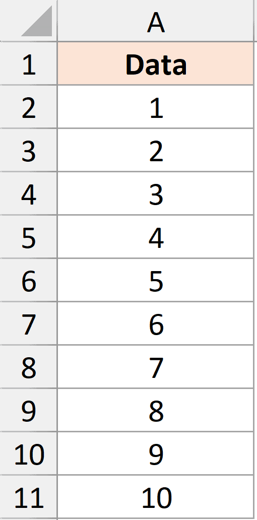
Below, I have a dataset where I have 10 numbers in A2:A11 and I want to add all of them.

Here is the SUM formula to do this:

=SUM(A2:A11)

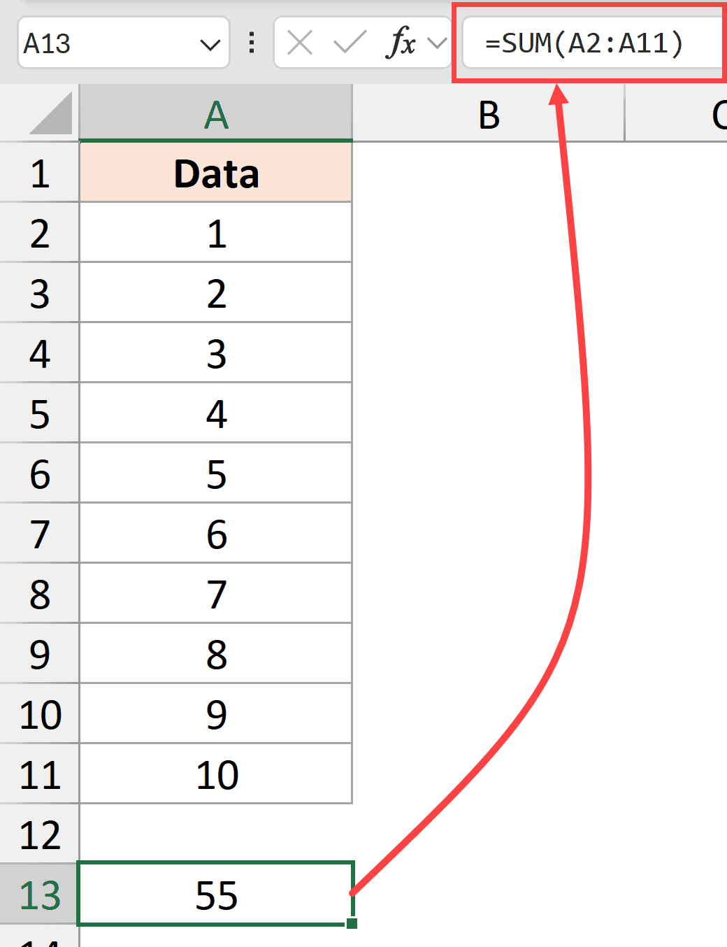
When you use the SUM formula, you probably think Excel just magically adds everything up and gives you the answer.

To understand the running total, imagine adding one value at a time:

• Step 1: Excel starts with 0
• Step 2: It looks at A2 and adds the number in A2 to 0
• Step 3: It takes that result and adds the value in A3 to it
• Step 4: It takes that result and adds the value in A4 to it
• …. and the steps continue till the last cell

Notice the pattern? Excel goes through each value, does something with it (adds it to the running total), carries that result forward, and repeats.

This is exactly how REDUCE function works in Excel.

The only difference is that instead of being stuck with the SUM function, REDUCE lets you decide what happens at each step.

Here’s SUM function recreated using the REDUCE function:

=REDUCE(0, A2:A11, LAMBDA(a, v, a + v))

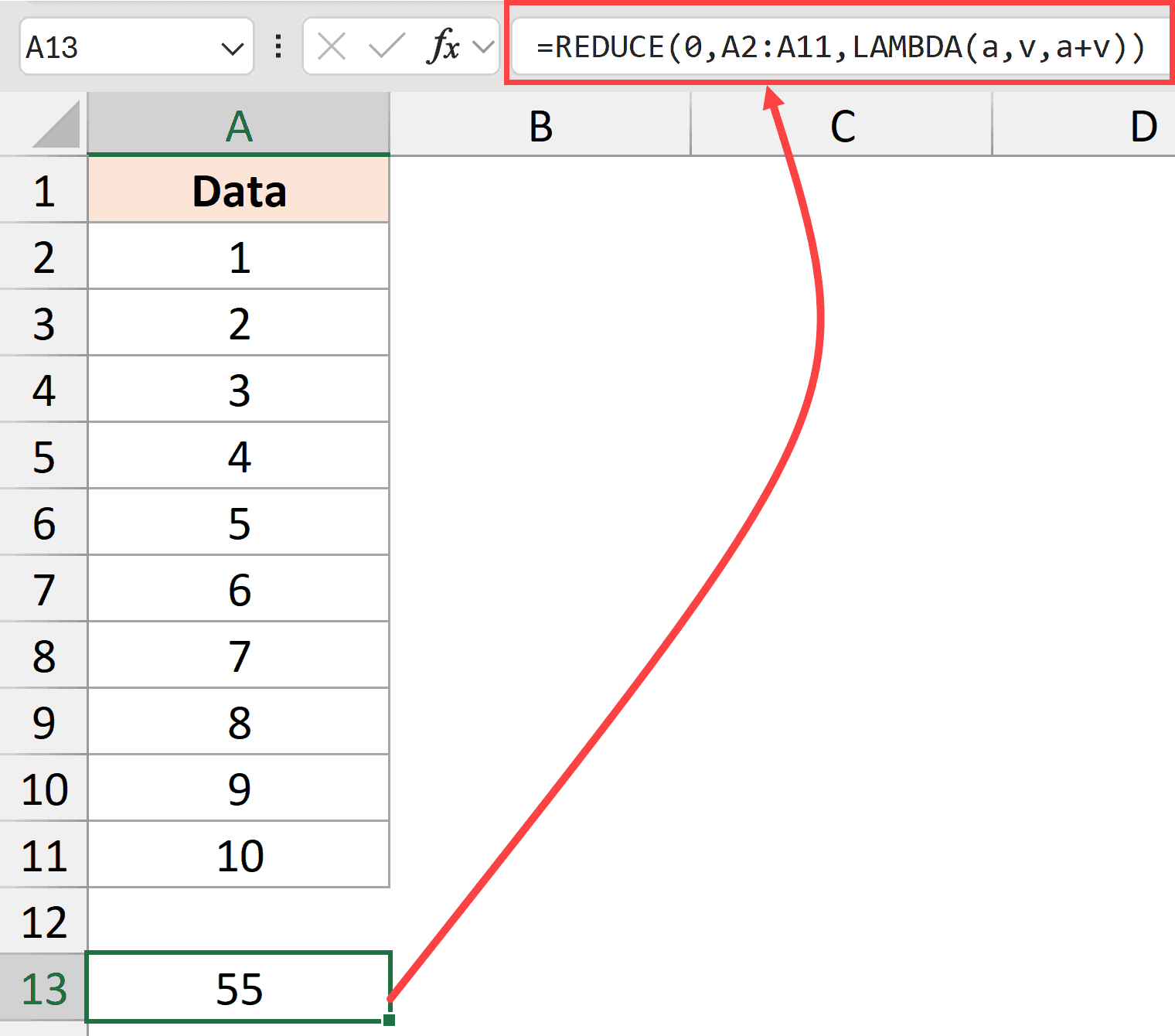
Let me break down what’s happening:

• 0 is your starting point (just like SUM starts with 0)
• A2:A11 is your range (same as SUM)
• a is your running result that carries forward. It starts with 0 (or whatever value is specified as the first argument of the REDUCE function), and after every step, the result of the Lambda function is assigned to this variable.
• v is the current cell being processed. So this would be A2 then A3 then A4 and so on.
• a + v is what happens within the lambda function

The formula goes:

• Start: total = 0
• Step 1: Look at A2 → Calculate 0 + 1 = 1 → Save 1 back into a
• Step 2: Look at A3 (which has 2) → Calculate 1 + 2 = 3 → Save 3 back into a
• Step 3: Look at A4 (which has 3) → Calculate 3 + 3 = 6 → Save 6 back into a
• …. continues till the last cell and the last calculation is then assigned to a
• The reduce function returns the value stored in a

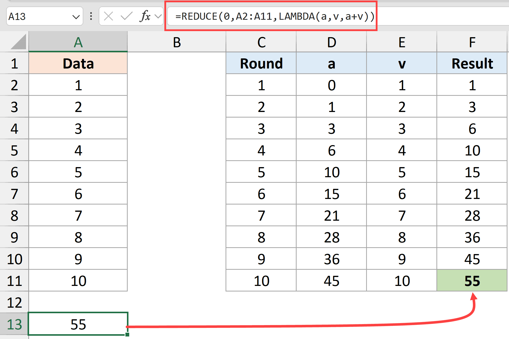
See what’s happening? At each step, REDUCE:

• Takes the current value from the accumulator (a)
• Performs your calculation with the current cell value (v)
• Saves that result back into the accumulator (a)
• Moves to the next cell and repeats

The accumulator is constantly being updated and carrying the result forward. That’s why it’s called an “accumulator”, as it accumulates the results as it goes.

Now here’s where it gets interesting.

Since you control what happens in that LAMBDA function, you can change the rules. Instead of simply adding the numbers, you can rewrite the lambda function to only add numbers that are greater than 5 (or create any LAMBDA you want).

This is what makes the REDUCE function so powerful.

Now let’s look at some practical examples of using the REDUCE function in Excel.

Note: If you omit the first argument in the REDUCE function, it will automatically take the first value in the specified range in the second argument.

Example 1: Conditional Sum using REDUCE

Below I have a dataset where I want to add all the numbers that are greater than 50.

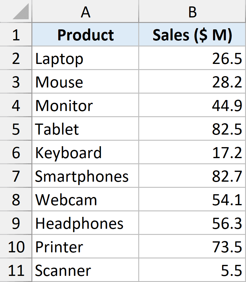
Now of course, you can do this using the SUMIF function. But let me still show you how to use the REDUCE function so that we can then use the same concept in more advanced examples later.

Here is the reduce formula that will do the conditional sum:

=REDUCE(0,B2:B11,LAMBDA(a,v,IF(v>50,a+v,a)))

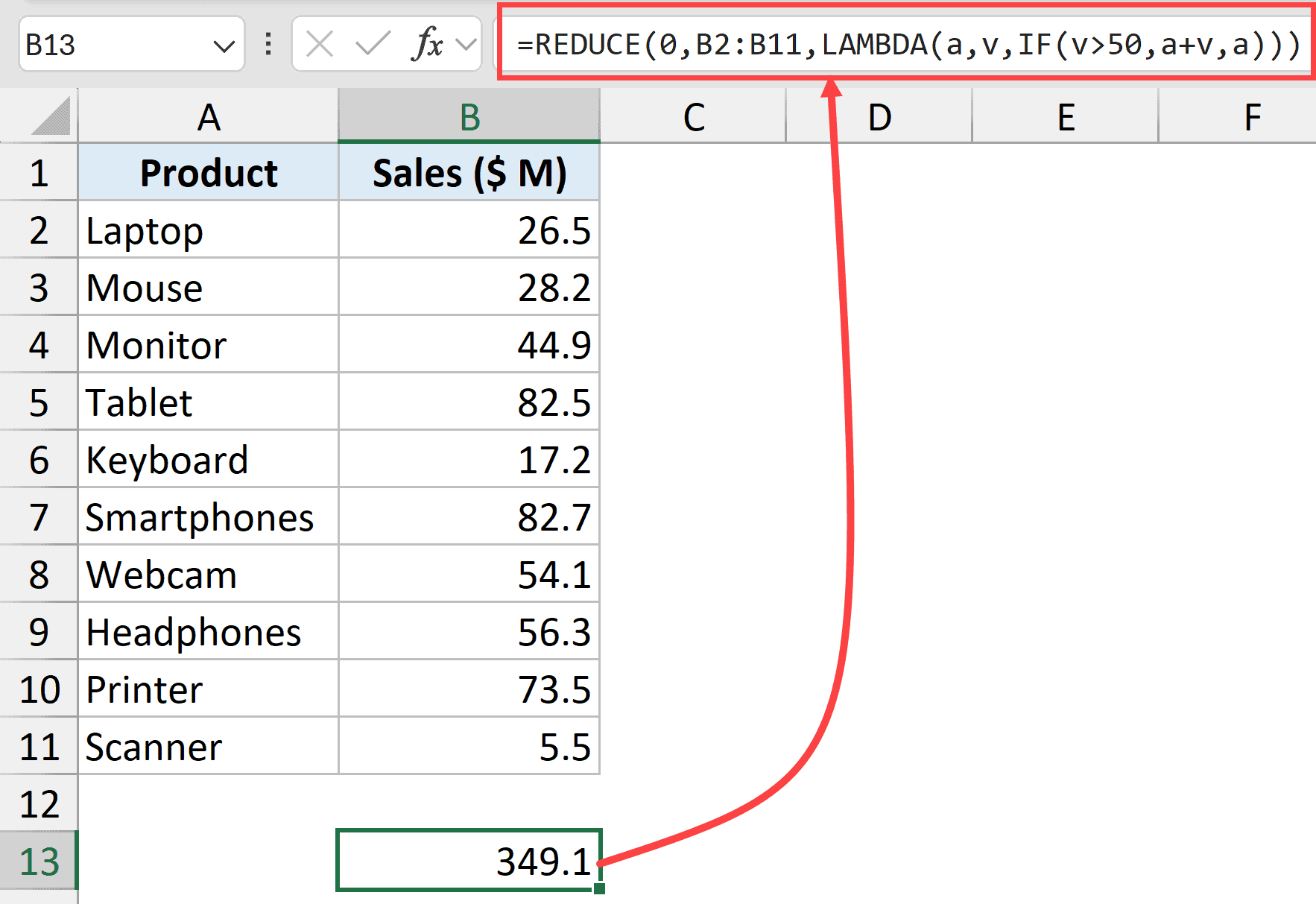
Here’s what’s happening in the formula:

• 0 – this is the first argument, which tells the function that the starting value is going to be 0.
• B2:B11 – this is the range on which the lambda function would be applied.
• LAMBDA(a,v,IF(v>50,a+v,a)) – this is the lambda function that does the conditional sum.
  • a – this is the accumulator value which starts with 0, and then holds the result after each cell is being processed by the lambda function.
  • v – this is the current value being processed by the lambda function.
  • IF(v>50,a+v,a) – this is the if condition that checks whether the value in the cell is more than 50 or not. If the value is more than 50, that value is added to the existing value in the accumulator variable (a), and if it is not more than 50, the previous accumulator value is returned as is.

Now that I have shown you two simple examples of using the REDUCE function, let’s move on to some advanced use cases.

Click here to download the example file

Example 2: Sum Sales by Region using REDUCE

Below I have a dataset where I have customer names in Column A and their order details in Column B.

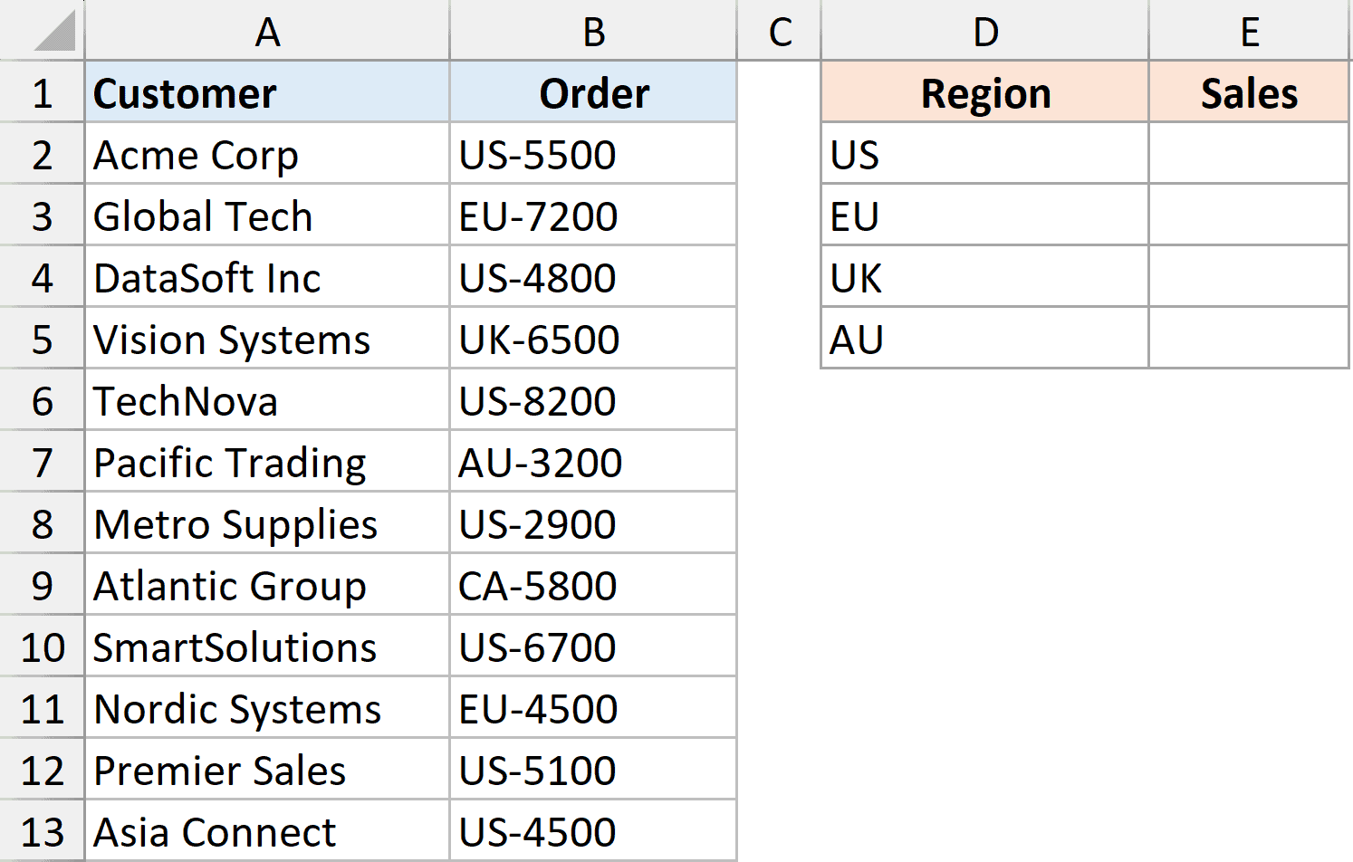
Note that the value of the order is preceded by a country code such as US-5500, which means that this order is from the US, and the value is 5500.

I want to fetch the total sales value by region and get the results in E2:E5.

Below is the formula that will do this.

=REDUCE(0,B2:B13,LAMBDA(a,v,IF(TEXTBEFORE(v,"-")=D2:D5,a+TEXTAFTER(v,"-"),a)))

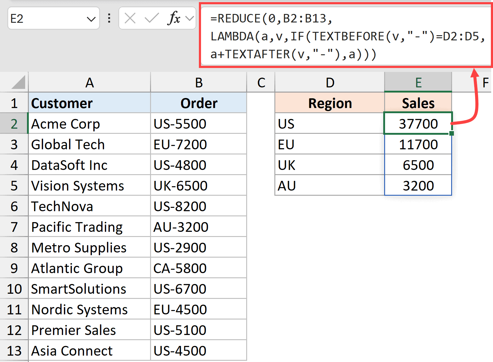
Here is what is happening in the above formula.

This example shows the accumulator becoming an array of regional totals. For routine grouping, parsed helper columns with SUMIF or a MAP/SUM approach can express the job more directly.

• 0 – this is the first argument, which tells the function that the starting value is going to be 0.
• B2:B13 – this is the range where we want to process each cell one-by-one.
• LAMBDA(a,v,IF(TEXTBEFORE(v,”-“)=D2:D5,a+TEXTAFTER(v,”-“),a)) – this is the lambda function that splits the country code and the numerical sales value and only adds the sales value for a given country.
  • a – this is the accumulator value which starts with 0, and then holds the result after each cell is being processed by the lambda function.
  • v – this is the current value being processed by the lambda function.
  • IF(TEXTBEFORE(v,”-“)=D2:D5,a+TEXTAFTER(v,”-“),a) – This checks the country code before the dash against D2:D5. TEXTAFTER extracts the sales amount after the dash and adds it to the matching country’s running total. The accumulator holds one total per country.

Example 3: Conditional Concatenation

Below I have a dataset where I have names in column A, and I want to concatenate and get all the names specific for each region in D2:D4

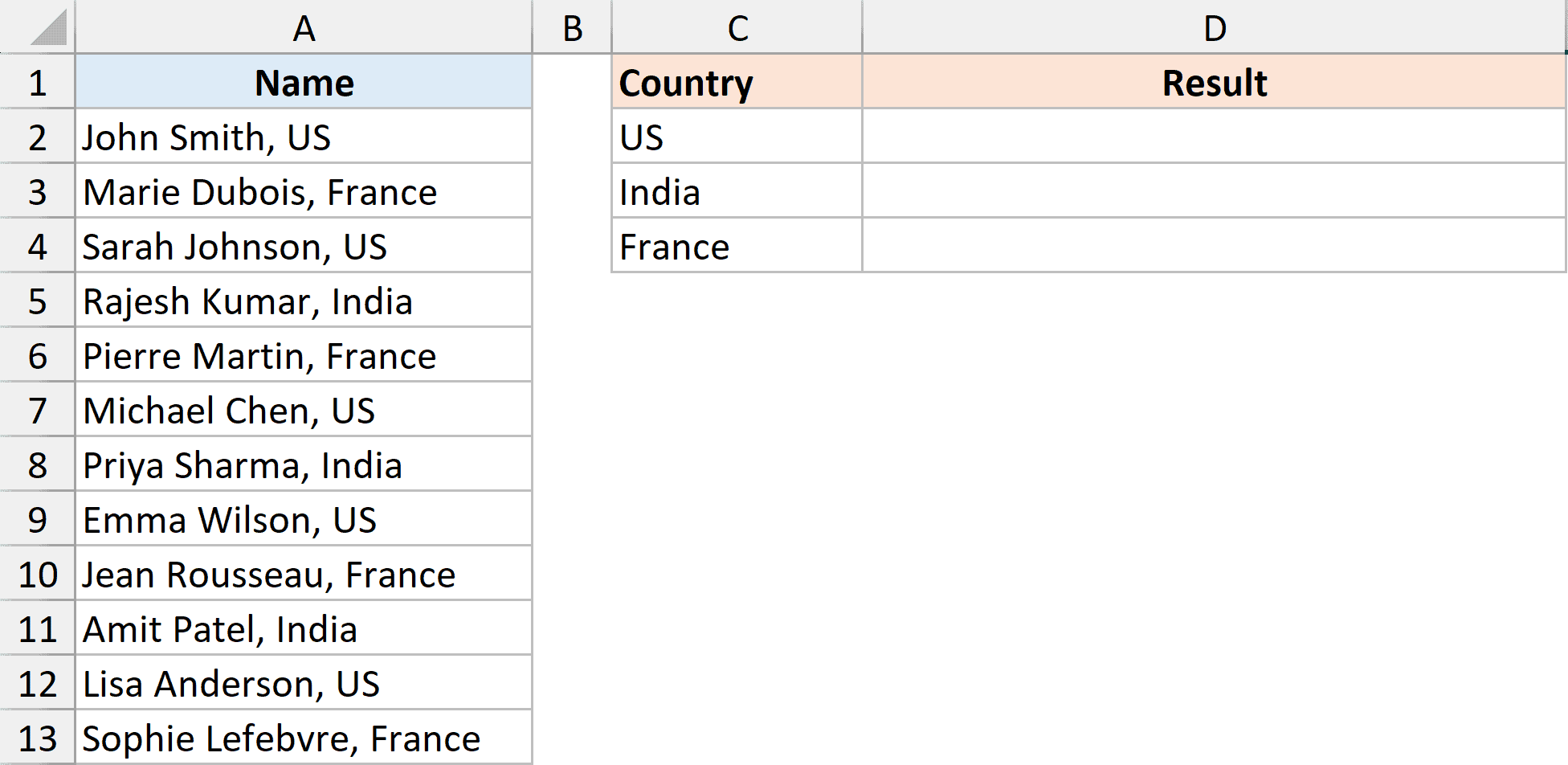
Below is the formula that will do this.

=SUBSTITUTE(REDUCE("",A2:A13,LAMBDA(a,v,IF(TEXTAFTER(v,", ")=C2:C4,a&", "&TEXTBEFORE(v,","),a))),", ","",1)

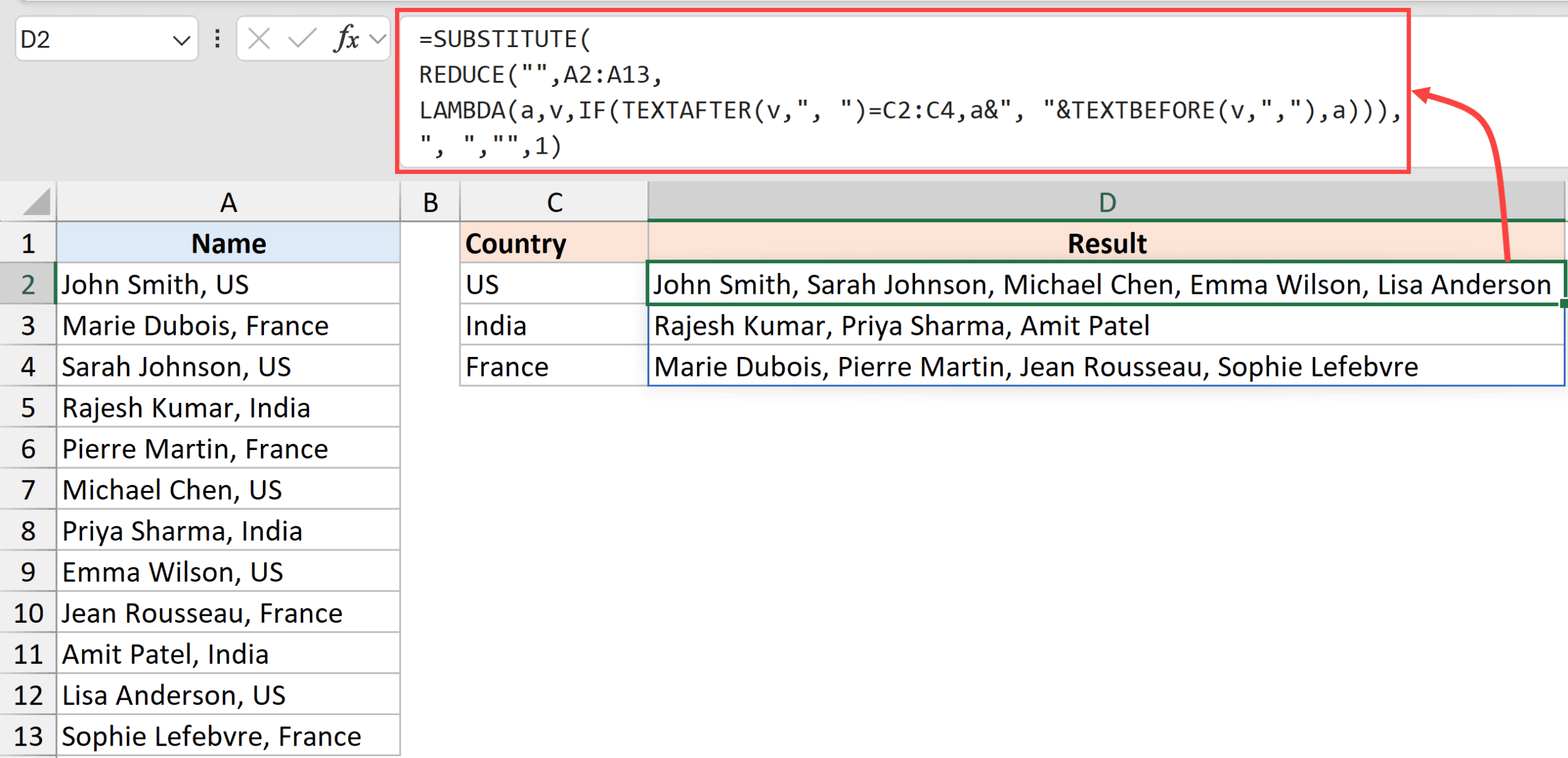
Here is what is happening within the REDUCE formula:

• “” – This is the first argument in the Reduce function. Since the expected output of this function is a text string, I am starting with a null string that will act as the starting point. Then, all the names for each country will be concatenated to this blank string.
• A2:A13 – this is the range where we want to process each cell one-by-one.
• LAMBDA(a,v,IF(TEXTAFTER(v,”, “)=C2:C4,a&”, “&TEXTBEFORE(v,”,”),a)) – this is the lambda function that uses an if condition to extract the country code after the name and based on that country code adds the name to the accumulator

In this example, each country’s result begins with a comma followed by a space character (“, “). So I’ve used the SUBSTITUTE function to remove the first instance of it from the final result.

This teaches an array of text accumulators. FILTER with TEXTJOIN is a more direct way to group names, without adding and then removing a leading separator.

Example 4: Text to Column with REDUCE

Below I have the address dataset in a comma-separated format, and I want to get each element of the address in a separate cell.

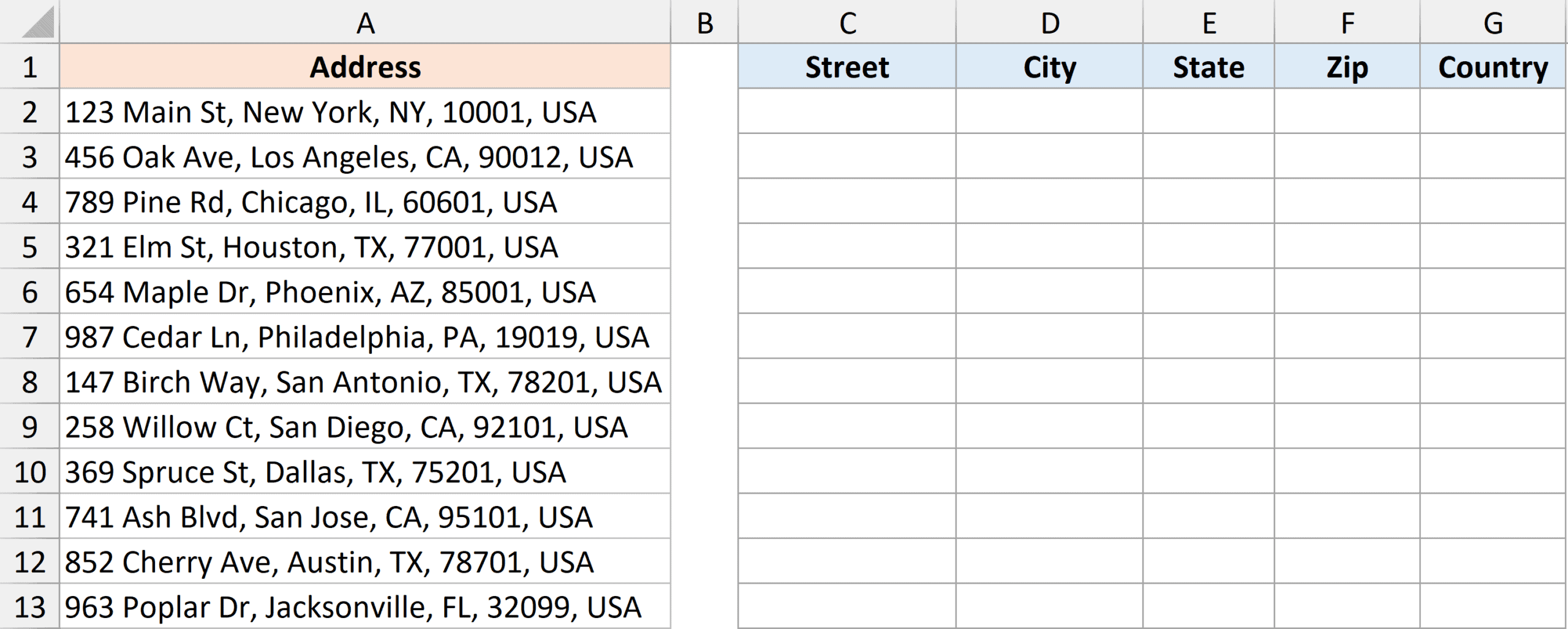
While I can use the TEXTSPLIT function to extract each element from a row, I cannot do it for the entire array in one go.

For example, I can use the below formula to get the first address split into separate columns.

=TEXTSPLIT(A2,", ")

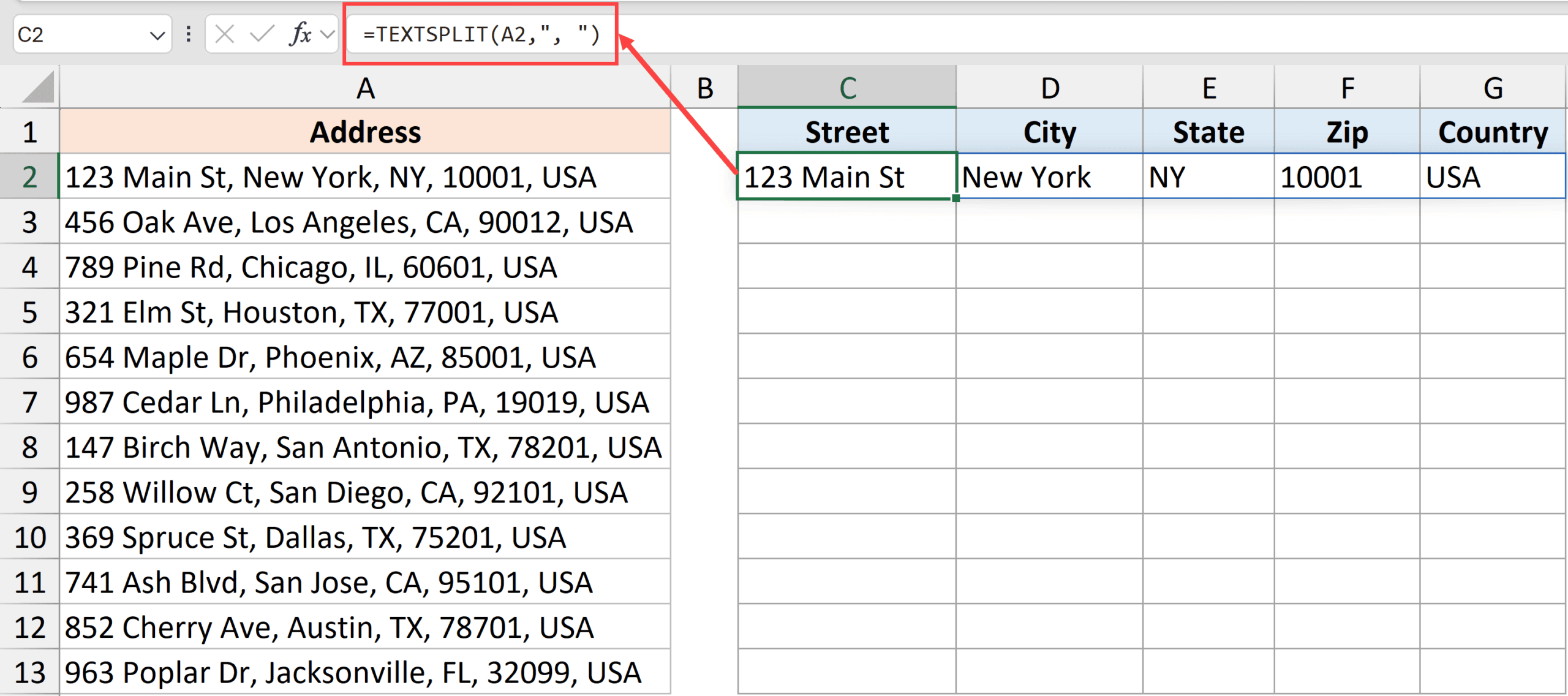
But it wouldn’t work if I use the below formula, where instead of A2, I use the entire range A2:A13.

=TEXTSPLIT(A2:A13,", ")

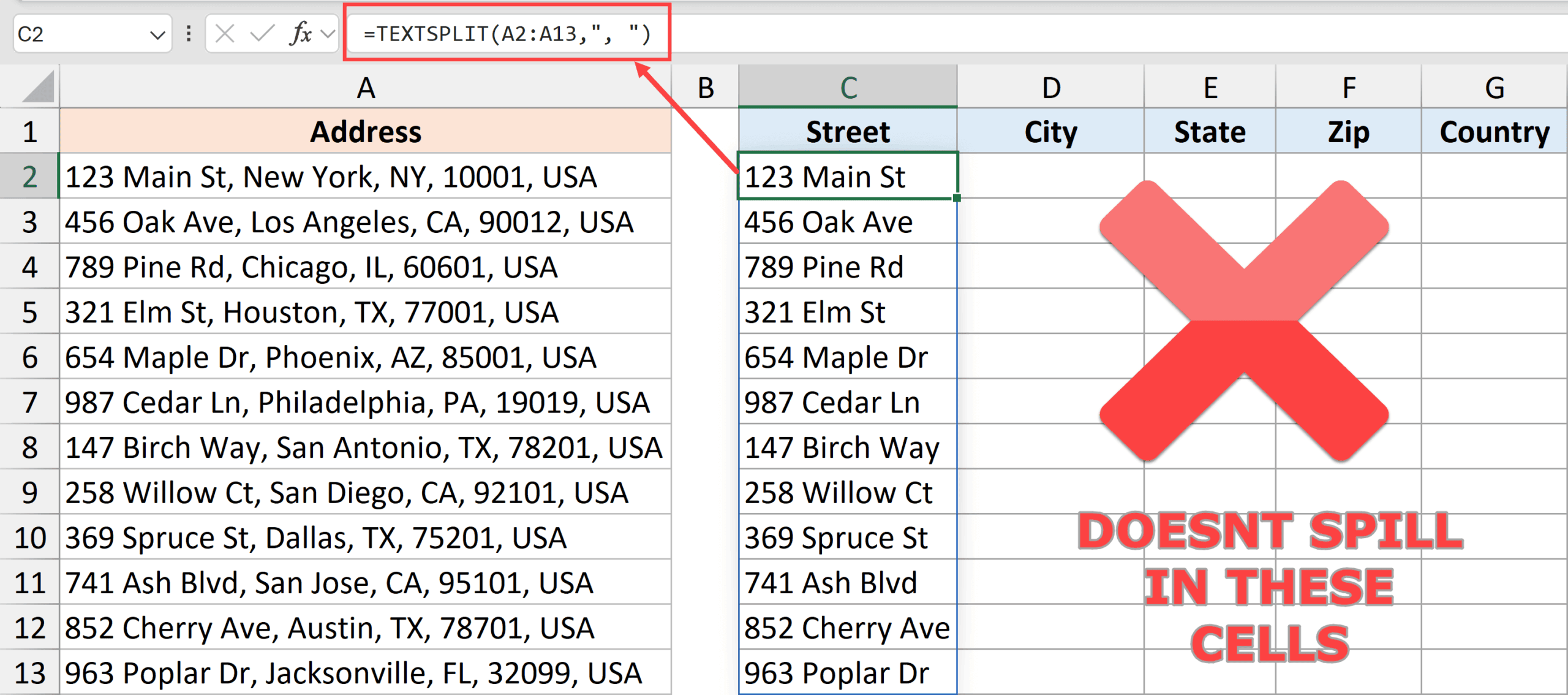
TEXTSPLIT can spill across both rows and columns. Here, passing A2:A13 directly doesn’t split each address into its own five-column row.

But if I want one single formula that would give me the entire result where all the addresses are split into separate cells, I can do that by using the below Reduce formula.

=DROP(REDUCE("",A2:A13,LAMBDA(a,v,VSTACK(a,TEXTSPLIT(v,", ")))),1)

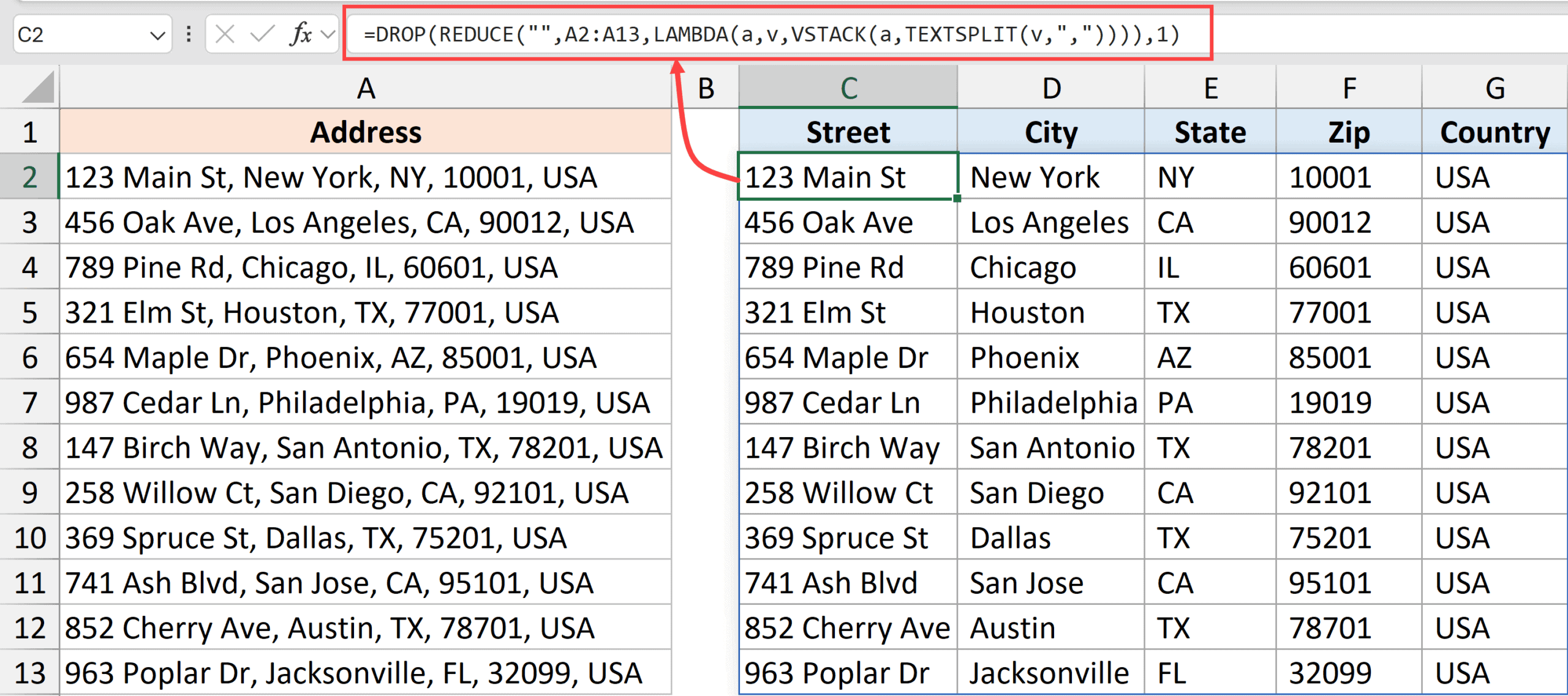
Here is what is happening in the above REDUCE formula.

• “” – I start with an empty string, which becomes the first row of the growing array.
• A2:A13 – this is the range where we want to process each cell one-by-one.
• LAMBDA(a,v,VSTACK(a,TEXTSPLIT(v,”, “)))
  • a – this is the accumulator value (starting with a “”).
  • v – this is the current value being processed by the lambda function.
  • VSTACK(a,TEXTSPLIT(v,”, “)) – The TEXTSPLIT function splits each address using a comma followed by a space as the delimiter. VSTACK adds that row of fields to the growing accumulator array.

Since I started with a null string as the initial value, VSTACK gives the result that has an extra row in the beginning that needs to be removed. This is done by using the DROP function.

Important: TEXTJOIN with TEXTSPLIT is shorter when the joined text fits within 32,767 characters. It also needs a row separator that doesn’t appear in the addresses.

REDUCE avoids that intermediate text limit, but repeated VSTACK calls copy a growing array and can slow down as the list grows.

Example 5: Find Unique Words in a Range

Below I have a movie genre dataset in column A, and I want to split the text in all the cells and get a list of unique words.

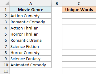
Below formula will do this

=DROP(UNIQUE(REDUCE("",A2:A10,LAMBDA(a,v,VSTACK(a,TEXTSPLIT(v,," "))))),1)

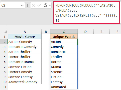
Here is what is happening in the above REDUCE formula.

• “” – I start with an empty string, which becomes the first row of the growing word array.
• A2:A10 – this is the range where we want to process each cell one-by-one.
• LAMBDA(a,v,VSTACK(a,TEXTSPLIT(v,,” “)))
  • a – this is the accumulator value (starting with a “”).
  • v – this is the current value being processed by the lambda function.
  • VSTACK(a,TEXTSPLIT(v,,” “)) – TEXTSPLIT splits each cell at spaces. Since the space is the row delimiter, the words spill vertically. VSTACK combines those words into one column. Multiword genres such as Science Fiction are split into separate words.

So, in short, the above REDUCE function is going to split and give us all the words in the selected range in one column.

Now, there are two things that need to be done – remove the first row containing our starting empty string, and remove all the duplicates.

This is done using the DROP function (which removes the first item from the result) and the UNIQUE function (which removes duplicates and gives only unique words).

Important: TEXTJOIN with TEXTSPLIT and UNIQUE is simpler when the joined text fits within 32,767 characters.

REDUCE avoids that intermediate text limit, but repeated stacking copies a growing array. This example assumes clean space-separated text, without blank cells or repeated spaces.

Click here to download the example file

Example 6: Bulk Find and Replace

This is an advanced example where REDUCE applies a sequence of replacements to a whole range of training codes.

Below I have a dataset where I have trainings done by people in column B, but these trainings use codes such as XL for Excel and PPT for PowerPoint.

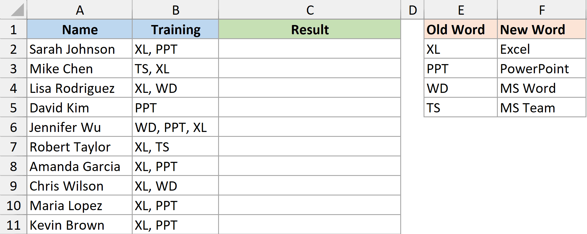
I want to replace these codes with actual training names (using the table in E1:F5).

In this example, REDUCE starts with the whole range B2:B11. It processes each code in E2:E5 in turn, replacing that code across the array using the table in E1:F5.

Below is the formula that will do this:

=REDUCE(B2:B11,E2:E5,LAMBDA(a,v,SUBSTITUTE(a,v,XLOOKUP(v,E2:E5,F2:F5))))

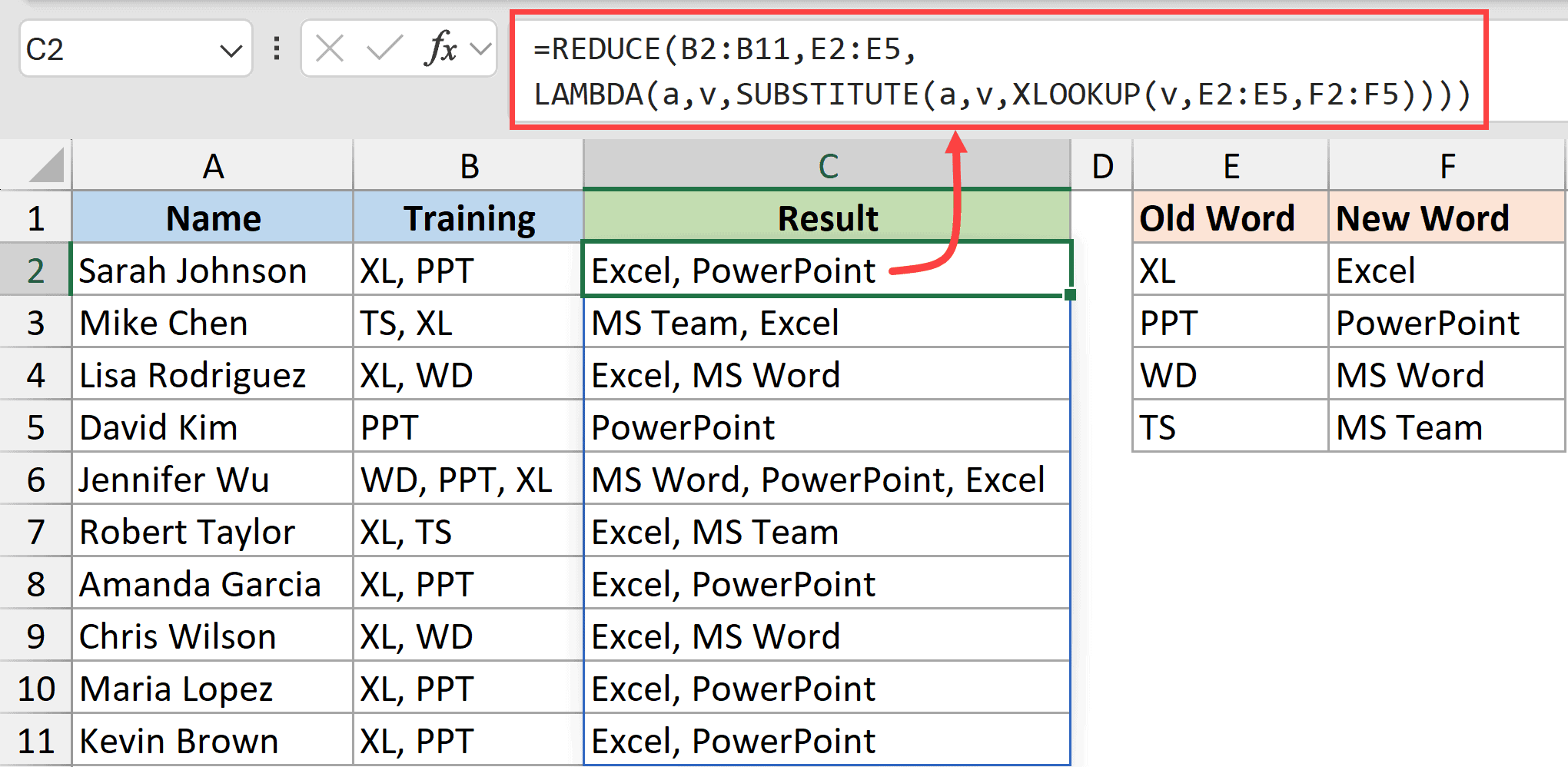
Let me explain what’s happening in this formula.

• B2:B11 – this range acts as the initial accumulator array. Each code replacement updates the whole array.
• E2:E5 – this is the range that will act as the current value for each iteration.
• LAMBDA(a,v,SUBSTITUTE(a,v,XLOOKUP(v,E2:E5,F2:F5)))
  • a – this is the accumulator array, which starts with all the values in B2:B11.
  • v – this is the current value (where the formula would process each cell in E2:E5)
  • SUBSTITUTE(a,v,XLOOKUP(v,E2:E5,F2:F5)) – XLOOKUP finds the full training name for the current code v. SUBSTITUTE replaces that code throughout the accumulator array a.

Since I’m using B2:B11 as the initial_value argument, the accumulator starts as a ten-row array. After all four code replacements, the final array spills down the column.

SUBSTITUTE matches text case-sensitively and can replace part of another code or cascade replacements with a different dictionary. For whole-code matching, a MAP/XLOOKUP approach is a more direct alternative.

Note: If this formula confuses you, just replace B2:B11 with B2 and see what you get. It will give you the result in one single cell only for the cell B2. And if you then replace B2 with B2:B11, it’ll give you the results for all the cells in this range

In this article, I’ve covered how to use the REDUCE function and covered some basic as well as advanced examples.

I hope you found this article helpful.

Below are some other Excel articles you may find useful:

• 10 VLOOKUP Examples For Beginner & Advanced Users
• 20 Advanced Excel Functions and Formulas (for Excel Pros)
• Split Text into Multiple Rows in Excel
• MAP Function in Excel (6 Examples)