

The BITAND function in Excel compares two numbers bit by bit and returns a number made up of only the bits that are 1 in both. It sounds nerdy (and it is a little), but it’s really handy when one number stores several yes/no options.
Some systems export data this way. Each option gets a value like 1, 2, 4, or 8, and a record’s code is the total of the options it has.
In this article, I’ll show you how BITAND works with six practical examples, including how to split a code into separate columns and how to find what two codes have in common.
Follow along with the example file
BITAND Function Examples.xlsx
BITAND Function Syntax
Here is the syntax of the BITAND function:
=BITAND(number1, number2)
- number1 – The first number. It must be a whole number that is 0 or more.
- number2 – The second number, with the same rules as number1.
BITAND turns both numbers into binary, compares them one position at a time, and keeps a 1 only where both numbers have a 1. You get the result back as a regular decimal number, not as binary.
Both numbers must be between 0 and 281,474,976,710,655 (that’s 2^48-1). A negative number or anything larger returns the #NUM! error.
BITAND also doesn’t round or cut off decimals for you. A number like 13.9, or a calculation like 0.5*7, returns #NUM!, so wrap it in INT or ROUND first.
Numbers stored as text, like “12”, work fine, and an empty cell counts as 0. Text that isn’t a number, like “abc”, returns the #VALUE! error.
The BITAND function works in Excel 2013 and later versions, including Microsoft 365, Excel 2024, 2021, 2019, 2016, and Excel for Mac.
When to Use the BITAND Function
Use this function when you need to:
- Check whether a specific option is included in a code that combines several options
- Check for a group of options at once, either all of them or any of them
- Split a combined code into separate columns, one per option
- Find what two codes have in common, like the days two people are both free
- Compare two numbers bit by bit and keep only the bits they share
Let me show you a few practical examples of how to use the BITAND function.
Example 1: Use BITAND to Compare Two Numbers
Let’s start with a simple example so you can see what BITAND does with plain numbers.
Below I have some pairs of numbers, and I want to get the BITAND result of each pair in column C.
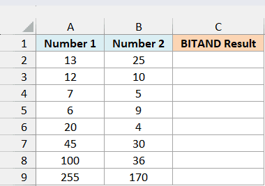
Here is the formula:
=BITAND(A2:A9,B2:B9)
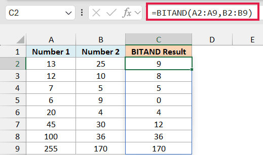
Enter this in cell C2, and it spills the results down to C9. BITAND goes row by row and compares the number in column A with the number in column B.
To see where the 9 in the first row comes from, here are 13 and 25 written in binary, with the value of each position at the top:
| Number | 16 | 8 | 4 | 2 | 1 |
|---|---|---|---|---|---|
| 13 | 0 | 1 | 1 | 0 | 1 |
| 25 | 1 | 1 | 0 | 0 | 1 |
| BITAND result | 0 | 1 | 0 | 0 | 1 |
Only the 8 and 1 positions have a 1 in both numbers, so BITAND returns 8 + 1 = 9.
That’s also why 6 and 9 return 0. In binary, 6 is 0110 and 9 is 1001, so they don’t share a single 1.
And when every 1 in one number is also in the other, like 36 and 100, you simply get the smaller number back.
If you want to see any number in binary like this, the BASE function can convert it for you.
If you are using Excel 2019 or earlier, enter the below formula in cell C2 and then copy it down the range:
=BITAND(A2,B2)
The formulas in Examples 2 and 3 work the same way. In Excel 2019 or earlier, enter them in the first result cell with B2 in place of B2:B11, and copy them down.
Example 2: Check If an Option Is Included in a Code
Now let’s look at where BITAND gets really useful.
Below is a list of hotel bookings where each guest’s extras are stored as one code, and I want to check whether each booking includes parking in column C.
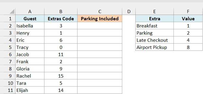
The table on the right shows the value of each extra. A booking’s code is the total of the extras it has, so Eric’s code of 6 means Parking (2) plus Late Checkout (4).
Here is the formula:
=IF(BITAND(B2:B11,2),"Yes","No")
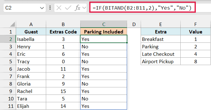
In the above formula, BITAND(B2:B11,2) keeps only the Parking part of each code. It returns 2 when parking is in the code and 0 when it isn’t.
The IF function treats any number other than 0 as TRUE, so a 2 gives you Yes and a 0 gives you No. For example, Jacob’s code of 11 is 8 + 2 + 1, so his booking includes parking.
To check a different extra, change the 2 to that extra’s value, like 8 for Airport Pickup.
Example 3: Check for Two Options at Once (All vs Any)
Here’s another practical scenario.
Below is a list of car rentals with an add-ons code for each renter, and I want to check which rentals have both GPS and Insurance in column C, and which have at least one of them in column D.
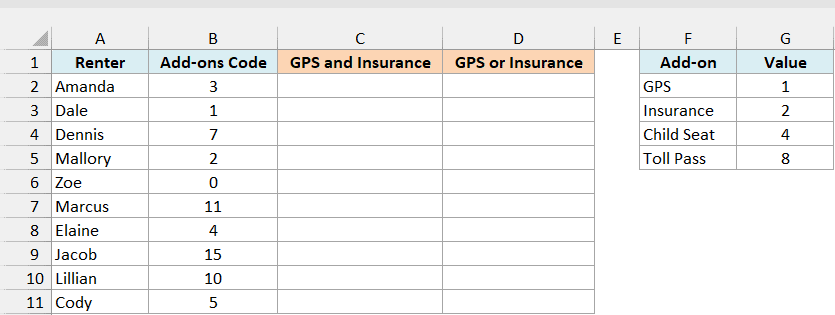
GPS is worth 1 and Insurance is worth 2, so a code that includes both of them has 1 + 2 = 3 inside it.
Here is the formula that checks for both:
=BITAND(B2:B11,3)=3
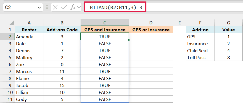
Here, the 3 works as a mask, which is just a number that holds the options you want to test for (GPS and Insurance).
BITAND(B2:B11,3) returns 3 only when both are in the code, so comparing it with 3 gives TRUE for the renters who have both.
Dennis has a code of 7 (GPS, Insurance, and Child Seat), so he gets TRUE. Mallory’s code of 2 has Insurance but no GPS, so she gets FALSE.
And here is the formula that checks for at least one of them:
=BITAND(B2:B11,3)>0
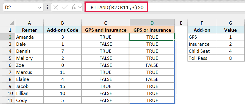
This time, the formula checks whether the result is more than 0, which happens when the code has GPS, Insurance, or both. Mallory now gets TRUE, while Zoe (0) and Elaine (4, Child Seat only) still get FALSE.
Pro Tip: To build a mask for any group of options, add up their values. For example, Insurance plus Toll Pass is 2 + 8 = 10, so you’d use 10 as the mask to check for both of them.
Example 4: Split a Code into Separate Columns
This next one turns each code into a row of checkmarks.
Below is a list of employees with a code for the days they work from the office, and I want to show a ✓ under each of their office days in columns C to G.
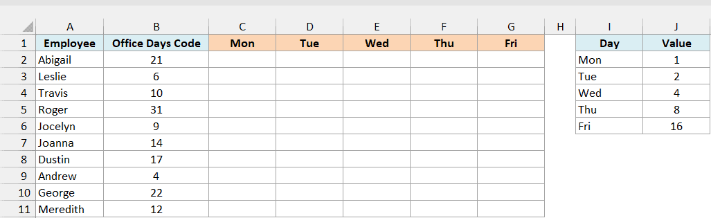
Monday is 1, Tuesday is 2, Wednesday is 4, Thursday is 8, and Friday is 16. So Abigail’s code of 21 is 1 + 4 + 16, which means Monday, Wednesday, and Friday.
Here is the formula:
=IF(BITAND(B2:B11,{1,2,4,8,16}),"✓","")
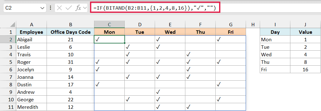
The {1,2,4,8,16} part is a list of the five day values, in the same order as the Mon to Fri headers. BITAND checks every code against every day value, so this one formula in C2 fills a grid 10 rows tall and 5 columns wide.
When a day is in the code, BITAND returns a number other than 0, and IF shows a ✓. Otherwise, IF returns an empty text (“”), so the cell looks blank.
Since this formula spills a whole grid, it needs Excel 365, 2024, or 2021.
Example 5: Filter Everyone Who Has a Specific Option
Let’s step it up and combine BITAND with the FILTER function.
Below is a list of summer camp registrations with an activities code for each camper, and I want to list all the campers who signed up for Soccer in column G.
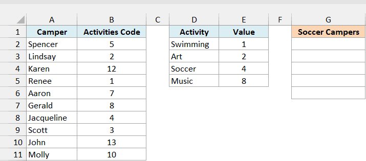
The table in the middle shows the value of each activity, and Soccer’s value of 4 is in cell E4.
Here is the formula:
=FILTER(A2:A11,BITAND(B2:B11,E4))
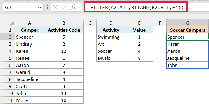
BITAND(B2:B11,E4) returns 4 for every camper whose code includes Soccer and 0 for everyone else.
FILTER treats the 4s as TRUE and the 0s as FALSE, so it keeps only the Soccer campers. Karen’s code of 12 is Soccer (4) plus Music (8), so she makes the list.
Since the formula points to E4 instead of a typed 4, you can change it to E2, E3, or E5 to list the campers for another activity.
The FILTER function works in Excel 365, 2024, and 2021.
Example 6: Find What Two Codes Have in Common
Let’s end with a more advanced use case, where you find the overlap between two codes and turn it back into day names.
Below is a tutoring schedule with the days each student is free and the days their tutor is free (both as codes), and I want to get the days they’re both free as a code in column D and as day names in column E.
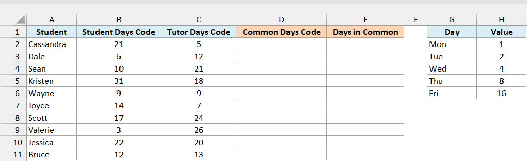
The day values are the same as in Example 4, with Monday as 1 and Friday as 16.
Here is the formula that gets the common days as a code:
=BITAND(B2:B11,C2:C11)
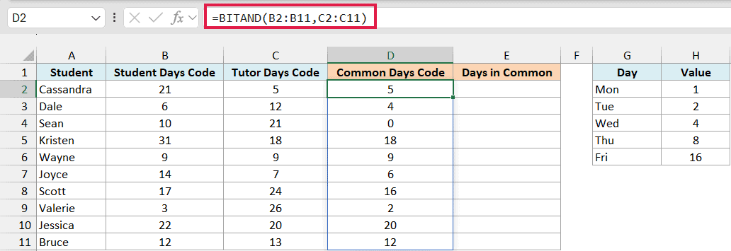
This compares each student’s code with their tutor’s code and keeps only the days that are in both. Cassandra is free on 21 (Mon, Wed, Fri) and her tutor on 5 (Mon, Wed), so they share 5, which is Monday and Wednesday.
Sean gets 0, because his free days (Tue, Thu) and his tutor’s free days (Mon, Wed, Fri) don’t overlap at all.
A result like Kristen’s 18 isn’t easy to read at a glance, so here is the formula that turns each common-days code into day names:
=MAP(D2#,LAMBDA(code,TEXTJOIN(", ",TRUE,FILTER({"Mon","Tue","Wed","Thu","Fri"},BITAND(code,{1,2,4,8,16}),"None"))))
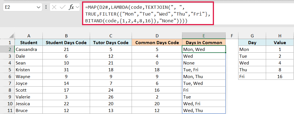
How this formula works:
- D2# refers to the whole spilled range of common-day codes from the previous formula.
- The MAP function goes through those codes one at a time and passes each one to the LAMBDA as code.
- BITAND(code,{1,2,4,8,16}) checks the code against each day value, just like in Example 4.
- FILTER keeps the day names where BITAND returned a number other than 0, and returns “None” when no day matches.
- TEXTJOIN combines the day names that are left into one text, separated by a comma and a space.
So Kristen’s code of 18 becomes “Tue, Fri”, and Sean’s 0 becomes “None”.
The MAP function works in Excel 365 and Excel 2024. If you are using Excel 2021, enter the below formula in cell E2 and then copy it down the range:
=TEXTJOIN(", ",TRUE,FILTER({"Mon","Tue","Wed","Thu","Fri"},BITAND(D2,{1,2,4,8,16}),"None"))
So these are some practical ways to use the BITAND function in Excel. Whenever your data packs several yes/no options into one number, BITAND lets you pull each option back out.
Just make sure both numbers are whole and not negative, or you’ll get the #NUM! error. I hope you found this article helpful.
Other Excel Articles You May Also Like:
