

The BITOR function in Excel compares two numbers in binary and returns a number that keeps every bit that is on in either of them. Put simply, it merges two numbers without counting anything twice.
That comes in handy when one number stores several yes/no options, with each option worth 1, 2, 4, 8, and so on. BITOR lets you combine two of these codes, or switch an option on, without messing up the code.
In this article, I’ll show you how BITOR works with five examples, from plain numbers to combining a whole column of codes into one.
Follow along with the example file
BITOR Function Examples.xlsx
BITOR Function Syntax
Here is the syntax of the BITOR function:
=BITOR(number1, number2)
- number1 – The first number. It must be a whole number that is 0 or more.
- number2 – The second number, with the same rules as number1.
BITOR writes both numbers in binary and checks them one position at a time. If either number has a 1 in a position, the result gets a 1 there, and you get the answer back as a regular decimal number.
Both numbers have to be between 0 and 281,474,976,710,655 (that’s 2^48-1). A negative number or anything bigger returns the #NUM! error.
BITOR also won’t drop decimals for you, so a number like 13.9 returns #NUM! instead of being treated as 13.
To fix this, wrap the number in the INT function, which drops the decimal part (13.9 becomes 13), like =BITOR(INT(A2),B2).
If you’d rather round to the nearest whole number (13.9 becomes 14), use the ROUND function instead, like =BITOR(ROUND(A2,0),B2).
Numbers stored as text, like “12”, work fine, and an empty cell counts as 0. Text that isn’t a number, like “abc”, returns the #VALUE! error.
The BITOR function works in Excel 2013 and later versions, including Microsoft 365, Excel 2024, 2021, 2019, 2016, and Excel for Mac.
When to Use the BITOR Function
Use this function when you need to:
- Combine two codes into one code that has every option from both
- Switch an option on in a code without changing the options already in it
- Add an option only to the records that meet a condition
- Combine a whole column of codes into a single code
- Compare two numbers bit by bit and keep every bit that is on in either one
Let me show you a few practical examples of how to use the BITOR function.
Example 1: Use BITOR on Two Numbers
Let’s start with plain numbers so you can see exactly what BITOR does.
Below I have some pairs of numbers, and I want to get the BITOR result of each pair in column C.
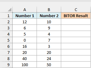
Here is the formula:
=BITOR(A2:A9,B2:B9)
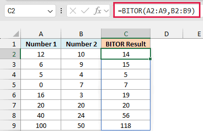
Enter this in cell C2, and it spills the results down to C9. BITOR takes the number in column A and the number in column B on each row and combines them.
To see where the 14 in the first row comes from, here are 12 and 10 written in binary, with the value of each position at the top:
| Number | 8 | 4 | 2 | 1 |
|---|---|---|---|---|
| 12 | 1 | 1 | 0 | 0 |
| 10 | 1 | 0 | 1 | 0 |
| BITOR result | 1 | 1 | 1 | 0 |
The 8, 4, and 2 positions have a 1 in at least one of the numbers, so BITOR returns 8 + 4 + 2 = 14.
Now look at the row with 5 and 4. In binary, 5 is 101 and 4 is 100, so the 4 is already inside the 5, and BITOR returns 5 (while 5 + 4 would give you 9).
The same thing happens with 20 and 20, which returns 20. BITOR never counts a bit twice, and that’s exactly what makes it useful in the examples that follow.
If you want to see any number in binary like this, the BASE function can convert it for you.
If you are using Excel 2019 or earlier, enter the below formula in cell C2 and then copy it down the range:
=BITOR(A2,B2)
Example 2: Combine Two Codes into One
Now let’s look at where BITOR gets really useful.
Below is a list of clothing items with one code for the sizes in stock at the store and another for the sizes in stock online, and I want the sizes available in either place as one code in column D.
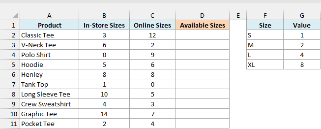
The table on the right shows the value of each size. A code is the total of the sizes it has, so the Hoodie’s in-store code of 5 means S (1) plus L (4).
Here is the formula:
=BITOR(B2:B11,C2:C11)
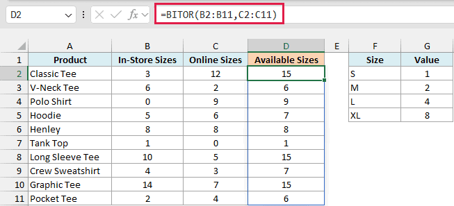
This combines each product’s in-store code with its online code. A size ends up in the result if it’s in either code.
Take the Hoodie. The store has S and L (5), and online has M and L (6), so the result is 7, which is S, M, and L.
L is in both codes, but BITOR counts it only once. If you added the two codes instead, you’d get 11, which reads as S, M, and XL, and makes it look like XL is in stock when it isn’t.
If you are using Excel 2019 or earlier, enter the below formula in cell D2 and then copy it down the range:
=BITOR(B2,C2)
Example 3: Add an Option to Every Code (BITOR vs Plus Sign)
Here’s a situation where using BITOR instead of plain addition makes a big difference.
Below is a list of gym members with a code for the perks in their plan, and since every member gets Sauna access this month, I want their new codes in column C.
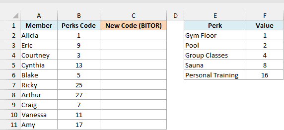
Sauna is worth 8 in the perks table. Some members already have it, like Eric, whose code of 9 is Gym Floor (1) plus Sauna (8).
Here is the formula:
=BITOR(B2:B11,8)
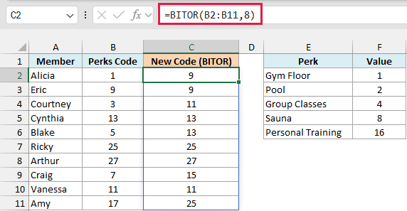
This switches the Sauna bit on in every code. Members who didn’t have Sauna get 8 more, and members who already had it keep the same code.
So Alicia’s code goes from 1 to 9, while Eric stays at 9 and Arthur stays at 27.
If you are using Excel 2019 or earlier, enter the below formula in cell C2 and then copy it down the range:
=BITOR(B2,8)
You might wonder why you can’t just add 8 to each code. Here is what that formula looks like:
=B2:B11+8
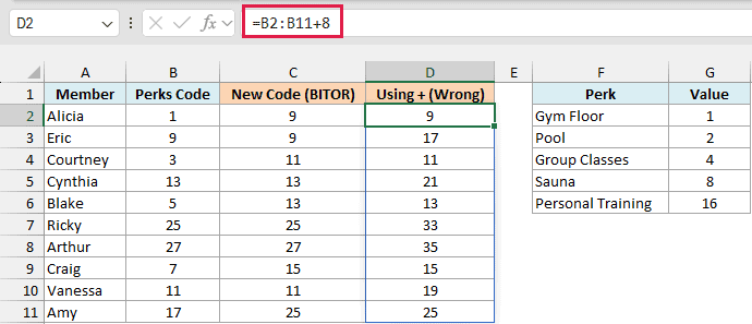
This works for members who didn’t have Sauna, but it breaks the code for everyone who did. Eric’s 9 becomes 17, which reads as Gym Floor plus Personal Training, so he loses Sauna and gets a perk he never had.
Ricky and Arthur end up with 33 and 35. Those codes are higher than all five perks added together (31), so they don’t match any real plan.
Important: Don’t use a plus sign to switch an option on in a code, because when the option is already there, the extra value carries over into another option. BITOR leaves the code as it is when the option is already in it.
Example 4: Add an Option Only When a Condition Is Met
Let’s step it up and combine BITOR with the IF function.
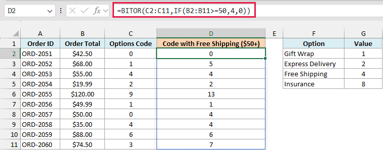
Below is a list of online orders with the order total and a code for the order options, and I want to add Free Shipping to every order of $50 or more, with the new codes in column D.
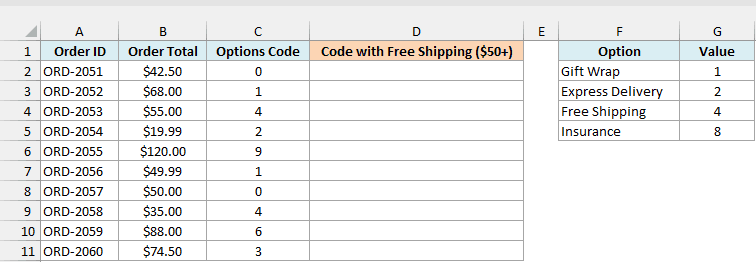
Free Shipping is worth 4 in the options table. Some orders already have it, like ORD-2058, even though it’s under $50.
Here is the formula:
=BITOR(C2:C11,IF(B2:B11>=50,4,0))
How this formula works:
- IF(B2:B11>=50,4,0) checks each order total and returns 4 (Free Shipping) when it’s $50 or more, and 0 when it’s less.
- BITOR then combines that number with the order’s options code.
- When IF returns 0, BITOR gives back the code unchanged, because combining a number with 0 doesn’t turn on any new bits.
So ORD-2052 ($68 with Gift Wrap) goes from 1 to 5, which is Gift Wrap plus Free Shipping. ORD-2057 is exactly $50, so it qualifies too and goes from 0 to 4.
ORD-2053 and ORD-2059 already had Free Shipping, so their codes stay the same. And ORD-2058 keeps the Free Shipping it already had, even though it’s under $50.
If you are using Excel 2019 or earlier, enter the below formula in cell D2 and then copy it down the range:
=BITOR(C2,IF(B2>=50,4,0))
Example 5: Combine a Whole Column of Codes into One
Let’s end with a more advanced use case, where you combine more than two codes at once.
Below is a list of ingredients in a banana bread recipe with an allergen code for each one, and I want a single allergen code for the whole recipe in cell G2.
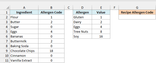
The table in the middle shows the value of each allergen. For example, Chocolate Chips has a code of 18, which is Dairy (2) plus Soy (16).
BITOR only takes two numbers, so it can’t combine a whole column on its own. That’s where the REDUCE function helps.
Here is the formula:
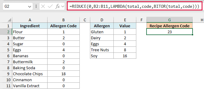
=REDUCE(0,B2:B11,LAMBDA(total,code,BITOR(total,code)))
How this formula works:
- The LAMBDA function inside REDUCE names two placeholders: total, which holds the running result, and code, which holds the current ingredient’s code.
- REDUCE starts total at 0, then goes through the codes in B2:B11 one at a time and passes each one to the LAMBDA as code.
- BITOR(total,code) combines the running total with the current code, and that becomes the new total.
- After the last ingredient, REDUCE returns the final total.
The result is 23, which is 16 + 4 + 2 + 1. So the recipe contains Soy, Eggs, Dairy, and Gluten.
If you used the SUM function on column B instead, you’d get 27, because Dairy shows up in Butter, Buttermilk, and Chocolate Chips. And 27 reads as Soy, Tree Nuts, Dairy, and Gluten, which wrongly adds Tree Nuts and leaves out Eggs.
The REDUCE function works in Excel 365 and Excel 2024. If you are using Excel 2021 or earlier, enter the below formula in cell C2 (with C1 left empty) and then copy it down to C11:
=BITOR(B2,C1)
Each cell combines one ingredient’s code with the result in the cell above it, so C11 ends up with the code for the whole recipe.
So these are some practical ways to use the BITOR function in Excel. Whenever you need to merge codes or switch an option on, BITOR does it without counting anything twice.
And when you need to check whether a code includes a specific option, that’s the job of its sibling, the BITAND function. I hope you found this article helpful.
Other Excel Articles You May Also Like:
