

The DECIMAL function in Excel converts a number written in another base, such as binary or hexadecimal, into a regular decimal number. You tell it the value and its base, and it gives you back a number you can calculate with.
It comes in handy when you get binary values, hex codes, or color codes from another system and need to work with them in Excel.
The one thing to watch is that the value has to use only the digits its base allows, or you get an error.
In this article, I’ll show you how the DECIMAL function works with six practical examples, from converting binary and hex values to turning color codes into RGB values.
Follow along with the example file
DECIMAL Function Examples.xlsx
DECIMAL Function Syntax
Here is the syntax of the DECIMAL function:
=DECIMAL(text, radix)
- text – The number you want to convert, written in the base you specify. It can be text in double quotes, a cell reference, or a plain number.
- radix – The base the number is written in. It should be a whole number from 2 to 36.
For bases above 10, the letters A to Z stand for the digits after 9, so A is 10, B is 11, and so on up to Z, which is 35. That’s why hex values (base 16) use the letters A to F.
A radix below 2 or above 36 returns the #NUM! error, since DECIMAL only supports bases 2 to 36.
If you give the radix a decimal value like 16.9, Excel drops the decimal part and uses 16.
The DECIMAL function works in Excel 2013 and later versions, including Excel 365, 2024, 2021, 2019, 2016, and Excel for Mac.
When to Use the DECIMAL Function
Use this function when you need to:
- Convert binary or hexadecimal values into regular numbers you can calculate with
- Turn hex color codes into their Red, Green, and Blue values
- Read a number written in any base from 2 to 36
- Convert hex or binary values longer than 10 characters, which HEX2DEC and BIN2DEC can’t handle
- Sort hex values by what they’re actually worth, not alphabetically
Let me show you a few practical examples of how to use the DECIMAL function in Excel.
Example 1: Convert Binary to Decimal in Excel
Let’s start with a simple example.
Below is a list of binary numbers, and I want to convert each one into a regular decimal number in column B.
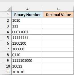
Here is the formula:
=DECIMAL(A2:A11,2)
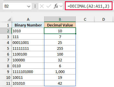
The radix 2 tells DECIMAL that the values in A2:A11 are binary. Since I gave it the whole range, one formula returns all ten results, and they spill into B2:B11 on their own.
Leading zeros don’t change the value, so 00011001 returns 25, the same as 11001 would.
The binary values here are stored as text to keep those zeros visible, but DECIMAL works just as well if you type a binary value like 1010 as a plain number.
Important: If a value has a space at the end, DECIMAL returns #NUM! for it, even though the cell looks fine. Wrap the range in TRIM to remove those spaces, like =DECIMAL(TRIM(A2:A11),2).
If you are using Excel 2019 or earlier, enter the below formula in cell B2 and then copy it down the column (the same approach works for Examples 2 and 5):
=DECIMAL(A2,2)
Example 2: Convert Hex to Decimal in Excel
Next, let’s convert hexadecimal (hex) values.
Below is a list of hex values, a few typed in lowercase and two with a 0x in front, and I want the decimal value of each one in column B.
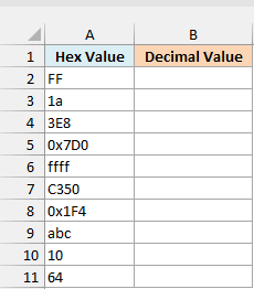
Here is the formula:
=DECIMAL(A2:A11,16)
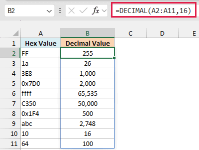
With 16 as the radix, DECIMAL reads every value as hex, and it doesn’t care about upper or lower case. So ffff returns 65,535, exactly what FFFF would.
The values with a 0x prefix also work. 0x is how programmers usually mark a hex number, and DECIMAL simply skips it, so 0x7D0 returns 2,000.
This only works when the radix is 16. With any other base, a 0x prefix returns #NUM!.
Excel’s older hex converter, the HEX2DEC function, returns #NUM! for 0x7D0, so this is one place where DECIMAL does better.
Also note that a hex value made of only digits is still hex. That’s why 10 returns 16 and 64 returns 100.
Example 3: Convert the Same Value From Different Bases
Here’s an example that shows what the radix argument does.
Below I have a few values in column A, and I want to see what each one is worth in base 2, 8, 10, 16, and 36, in columns B to F.
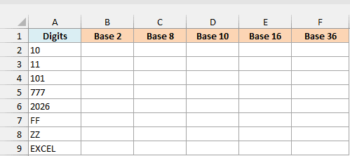
Here is the formula:
=DECIMAL(A2:A9,{2,8,10,16,36})
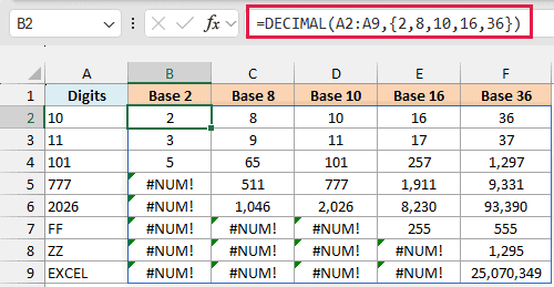
Instead of one radix, I gave DECIMAL five of them in curly brackets. It reads every value in A2:A9 in each of those bases, and the whole grid of results spills from B2.
Notice how the same digits mean different numbers. 101 is 5 in binary, 65 in base 8, and 257 in hex.
The #NUM! errors show up where a value uses a digit its base doesn’t have. Binary only has 0 and 1, so 777 can’t be binary, and FF needs base 16 or higher because F stands for 15.
ZZ only works in base 36, since Z (35) is the biggest digit there is.
And yes, even the word EXCEL is a valid base 36 number. It works out to 25,070,349.
Example 4: Convert Hex Color Codes to RGB Values
Let’s step it up with something you might actually run into when working with website or brand colors.
Below is a list of website elements with their hex color codes, and I want the Red, Green, and Blue values for each one in columns C, D, and E.
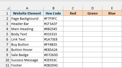
Here is the formula:
=DECIMAL(MID(B2:B11,{2,4,6},2),16)
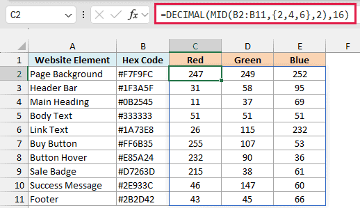
How this formula works:
- A hex color code like #1A73E8 is three pairs of hex digits after the #. The first pair (1A) is red, the second (73) is green, and the third (E8) is blue.
- MID(B2:B11,{2,4,6},2) uses the MID function to pull out two characters starting at positions 2, 4, and 6 of each code, which skips the #.
- DECIMAL(…,16) then converts each of those pairs from hex, so #1A73E8 gives 26, 115, and 232.
- Since there are ten codes and three pairs in each, the results spill into a ten-row, three-column block from C2 to E11.
Important: The # is not a hex digit, so feeding a full color code like #1E90FF straight into DECIMAL returns #NUM!. This formula also expects six-digit codes, so expand a short code like #FFF to #FFFFFF first.
If you are using Excel 2019 or earlier, enter the below formula in cell C2, copy it across to E2, and then copy it down to row 11:
=DECIMAL(MID($B2,2*COLUMNS($C2:C2),2),16)
Here, COLUMNS($C2:C2) returns 1, 2, and 3 as you copy the formula across, so MID starts at position 2 for red, 4 for green, and 6 for blue.
Example 5: DECIMAL vs HEX2DEC for Long Hex Values
You saw the HEX2DEC function briefly in Example 2, so it’s fair to ask why you’d use DECIMAL for hex at all. This example shows the difference.
Below is a list of hex values that get longer as you go down, and I want the decimal value of each one in column B.
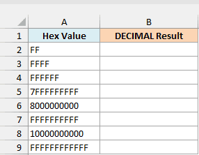
Here is the formula:
=DECIMAL(A2:A9,16)
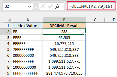
DECIMAL returns the correct value for every row, including the 12-character FFFFFFFFFFFF, which is 281,474,976,710,655.
Now here is the HEX2DEC formula in column C for comparison. I’ve entered it in C2 and copied it down, because HEX2DEC is one of the functions that won’t spill and returns #VALUE! when you give it a whole range:
=HEX2DEC(A2)
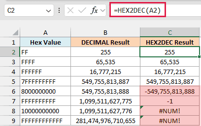
The first four rows match. But HEX2DEC only takes up to 10 characters, so the 11 and 12-character values return #NUM!.
The bigger problem is the 10-character values that start with 8 to F. HEX2DEC reads those as negative numbers, which is why 8000000000 returns -549,755,813,888 and FFFFFFFFFF returns -1.
DECIMAL has a limit too, but it’s much higher. Results above 9,007,199,254,740,991 lose precision, so a hex value longer than 13 characters may come back slightly off.
Important: If your values can be 10 characters or longer, use DECIMAL instead of HEX2DEC (the same goes for BIN2DEC and OCT2DEC). A negative result looks like a real number, so this mistake is easy to miss.
Example 6: Sort Hex Values by Their Actual Value
Here’s one last practical use, where DECIMAL works behind the scenes inside another formula.
Below is a list of hex values in random order, and I want them sorted from the smallest value to the largest in column B.
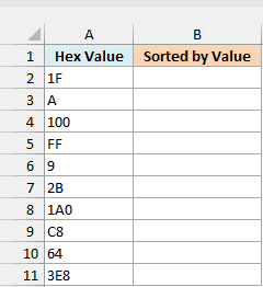
If you sort these with the SORT function, Excel treats them as text and sorts them alphabetically. That puts 100 before 9 and leaves FF at the very end, even though 100 is the bigger number.
Here is the formula that sorts them by value:
=SORTBY(A2:A11,DECIMAL(A2:A11,16))
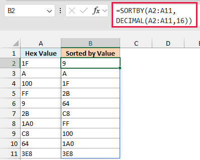
Here, DECIMAL(A2:A11,16) converts every hex value to a number, and SORTBY uses those numbers to sort the original list.
The converted numbers never show up on the sheet. You only see the hex values in the right order, from 9 up to 3E8 (which is 1,000).
The SORTBY function is only available in Excel 2021 and later versions, including Microsoft 365. If you are using Excel 2019 or earlier, enter the below formula in cell C2, copy it down, and then sort the data by column C:
=DECIMAL(A2,16)
So that’s how you can use the DECIMAL function in Excel to turn binary, hex, and other base values into regular numbers. It’s also the safer choice over HEX2DEC once your hex values get long.
If you need to go the other way and turn a decimal number into binary or hex, that’s the job of the BASE function.
I hope you found this tutorial useful.
Other Excel Articles You May Also Like:
