

The BITRSHIFT function in Excel moves the bits of a number (the 1s and 0s you get when you write it in binary) to the right by the number of positions you tell it. It then gives you the result as a regular decimal number.
Each position you shift halves the number and drops any remainder.
It’s most useful when one number has several smaller values packed inside it. A good example is the number Excel uses to store a color, which holds the red, green, and blue values together.
In this article, I’ll show you how BITRSHIFT works with five practical examples, from shifting a few plain numbers to splitting a color code into its red, green, and blue parts.
Follow along with the example file
BITRSHIFT Function Examples.xlsx
BITRSHIFT Function Syntax
Here is the syntax of the BITRSHIFT function:
=BITRSHIFT(number, shift_amount)
- number – The number whose bits you want to shift. It must be a whole number that is 0 or more.
- shift_amount – How many positions to shift the bits to the right. It must be a number between -53 and 53.
BITRSHIFT turns the number into binary, removes as many digits from the right end as the shift_amount says, and converts what’s left back to a decimal number.
The number can be anything from 0 to 281,474,976,710,655 (that’s 2^48-1). A negative number, a number above that limit, or a shift_amount beyond 53 either way returns the #NUM! error.
The number also has to be a whole number. Something like 13.9 returns #NUM!, so wrap it in the INT function or the ROUND function first if your values can have decimals.
The shift_amount is more forgiving. A decimal like 1.9 is simply cut down to 1, so it shifts by one position.
A negative shift_amount shifts the bits to the left instead of the right. Example 2 shows how that works.
Numbers stored as text, like “12”, work fine, and an empty cell counts as 0. Text that isn’t a number, like “abc”, returns the #VALUE! error.
The BITRSHIFT function works in Excel 2013 and later versions, including Microsoft 365, Excel 2024, 2021, 2019, 2016, and Excel for Mac.
When to Use the BITRSHIFT Function
Use this function when you need to:
- Shift the bits of a number to the right and get the result as a decimal number
- Divide a number by 2, 4, 8, or any power of 2 and drop the remainder
- Read the individual bits (the 1s and 0s) of a number
- Count how many options are turned on in a code that combines several options
- Pull out a value that’s packed inside a larger number, like the red, green, and blue parts of a color code
Let me show you a few practical examples of how to use the BITRSHIFT function.
Example 1: Shift Numbers to the Right with BITRSHIFT
Let’s start with a simple example so you can see what BITRSHIFT does with plain numbers.
Below I have some numbers with a shift amount next to each, and I want to get the shifted result of each one in column C.
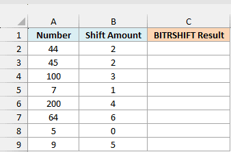
Here is the formula:
=BITRSHIFT(A2:A9,B2:B9)
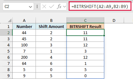
Enter this in cell C2, and it spills the results down to C9. BITRSHIFT goes row by row and shifts the number in column A by the amount in column B.
To see where the 11 in cell C2 comes from, here is 44 written in binary, before and after the shift, with the value of each position at the top:
| 32 | 16 | 8 | 4 | 2 | 1 | |
|---|---|---|---|---|---|---|
| 44 | 1 | 0 | 1 | 1 | 0 | 0 |
| Shifted right by 2 | 0 | 0 | 1 | 0 | 1 | 1 |
The two digits on the right (0 and 0) fall off, and everything else moves two places to the right. What’s left is 1011, which is 8 + 2 + 1 = 11.
Now look at row 3. 45 is 101101 in binary, so shifting it by 2 drops a 0 and a 1, which also leaves 1011.
That’s why 44 and 45 both return 11, because the bits that fall off are gone for good.
Another way to think about it is that every shift to the right halves the number and throws away any remainder. So shifting 100 by 3 is the same as 100 divided by 8, which is 12.5, and BITRSHIFT returns 12.
A shift amount of 0 gives you the same number back, like the 5 in row 8.
And if you shift by more positions than the number has binary digits, you get 0. That’s what happens with 9 (binary 1001) shifted by 5.
If you want to see any number in binary like this, the BASE function can convert it for you.
If you are using Excel 2019 or earlier, enter the below formula in cell C2 and then copy it down the range:
=BITRSHIFT(A2,B2)
Example 2: Use a Negative Shift Amount to Shift Left
This next one might surprise you, since BITRSHIFT is meant to shift bits to the right.
Below I have some numbers with negative shift amounts, and I want to get the BITRSHIFT result of each one in column C.
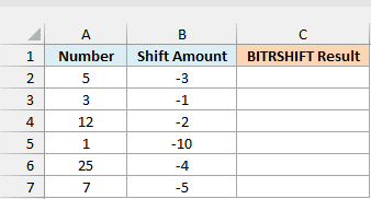
Here is the formula:
=BITRSHIFT(A2:A7,B2:B7)
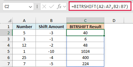
When the shift amount is negative, BITRSHIFT shifts the bits to the left and adds 0s on the right. Each position to the left doubles the number.
So 5 (binary 101) shifted by -3 becomes 101000, which is 40. That’s the same as 5 multiplied by 2 three times.
In the same way, 1 shifted by -10 gives you 1024.
This works exactly like the BITLSHIFT function with a positive shift amount, so BITRSHIFT(5,-3) and BITLSHIFT(5,3) both return 40.
When you shift left, the result can’t go past 281,474,976,710,655 (2^48-1). If it would, BITRSHIFT returns the #NUM! error.
If you are using Excel 2019 or earlier, enter the below formula in cell C2 and then copy it down the range:
=BITRSHIFT(A2,B2)
Example 3: Show Each Number’s Binary Digits in Separate Columns
Now let’s look at a more useful way to use BITRSHIFT, where you read the bits of a number one at a time.
Below I have a list of numbers, and I want to show each number’s eight binary digits in columns B to I, one digit per column.
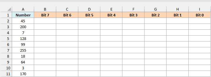
The headers in row 1 show “Bit 7” to “Bit 0”, but the cells actually hold the numbers 7 to 0. They’re the bit positions, counted from 0 on the far right, and the “Bit” label is just a custom number format.
Here is the formula:
=BITAND(BITRSHIFT(A2:A11,B1:I1),1)
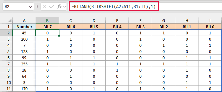
This one formula in B2 fills a grid that’s 10 rows tall and 8 columns wide.
How this formula works:
- BITRSHIFT(A2:A11,B1:I1) shifts every number by each of the positions in row 1, from 7 down to 0. Shifting by a position moves the bit at that position all the way to the right end.
- The BITAND function with 1 keeps only that rightmost bit and drops everything else, so each cell ends up with a 1 or a 0.
For example, 45 is 00101101 as an 8-digit binary number, and that’s exactly what you see across row 2. You can read 170 in the last row as 10101010 the same way.
Since the headers in B1:I1 are the shift amounts, they have to stay numbers. If you type “Bit 7” into B1 as text, every result in column B shows the #VALUE! error.
Since this formula spills a whole grid, it needs Excel 365, 2024, or 2021. If you are using Excel 2019 or earlier, enter the below formula in cell B2 and then copy it across to column I and down to row 11:
=BITAND(BITRSHIFT($A2,B$1),1)
Example 4: Count the Options in a Combined Code
Here’s another practical scenario.
Below is a list of pizza orders where the toppings are stored as one code, and I want to count how many toppings each order has in column C.
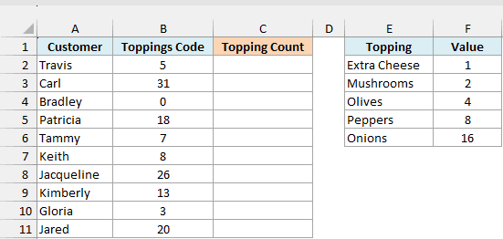
The table on the right shows the value of each topping, just for reference. An order’s code is the total of the toppings in it, so Travis’s code of 5 means Extra Cheese (1) plus Olives (4).
Here is the formula:
=SUM(BITAND(BITRSHIFT(B2,{0,1,2,3,4}),1))
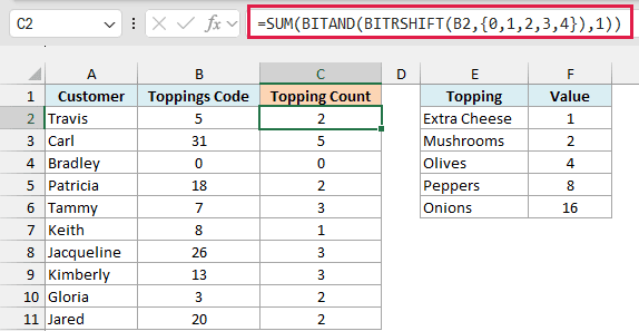
Enter this in cell C2 and copy it down to C11.
How this formula works:
- Each topping value is a power of 2, so it takes up exactly one binary digit. Extra Cheese (1) is position 0, Mushrooms (2) is position 1, Olives (4) is position 2, Peppers (8) is position 3, and Onions (16) is position 4.
- BITRSHIFT(B2,{0,1,2,3,4}) shifts the code by each of those positions, which brings each topping’s bit to the right end in turn.
- BITAND(…,1) turns each of those five results into a 1 (topping included) or a 0 (not included).
- The SUM function adds up the 1s, which gives you the number of toppings.
So Carl’s code of 31 returns 5 because he has all five toppings. Jacqueline’s 26 is 16 + 8 + 2 (Onions, Peppers, and Mushrooms), so she gets 3.
If you add a sixth topping with a value of 32 (position 5), add its position to the list as well, so it becomes {0,1,2,3,4,5}. Otherwise the formula won’t count it.
Here we keep this as a per-row formula because SUM adds everything it gets into one number. If you gave it the whole range B2:B11, you’d get one total for all the orders instead of a count for each.
Example 5: Split an Excel Color Code into Red, Green, and Blue
Let’s end with a more advanced use case, where a number has three values packed inside it.
Below is a list of Excel’s standard colors with the color code Excel uses for each, and I want to get the red, green, and blue values of each color in columns C, D, and E.
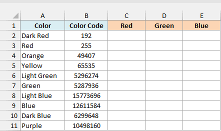
Excel stores a color as one number, where Red is the first 8 bits on the right, Green is the next 8 bits, and Blue is the 8 bits after that.
If you’ve used VBA, this is the number you get back from a cell’s Interior.Color property.
Here is the formula:
=BITAND(BITRSHIFT(B2:B11,{0,8,16}),255)
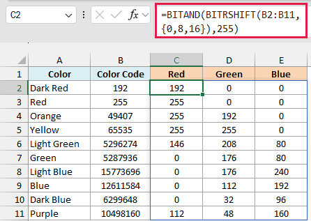
Enter this in cell C2, and it spills across to column E and down to row 11.
How this formula works:
- BITRSHIFT(B2:B11,{0,8,16}) shifts each color code by 0, 8, and 16 positions. That brings the Red, Green, and Blue values to the right end, one at a time.
- BITAND(…,255) keeps only the last 8 bits (255 is 11111111 in binary), so you get just that one color value, from 0 to 255.
Since the {0,8,16} part has three values, the formula spills into three columns as well as ten rows.
Light Green’s code of 5296274 becomes 146, 208, and 80, which are the same red, green, and blue values you’d see for that color in the More Colors dialog box.
Because this formula spills a whole grid, it needs Excel 365, 2024, or 2021.
If your colors are hex codes like #92D050 instead, the DECIMAL function can turn each pair of hex digits into its red, green, and blue value.
So these are some practical ways to use the BITRSHIFT function in Excel. In most of them, the idea is the same: shift the bits you want to the right end, then keep only those bits with BITAND.
Just make sure the number is whole and not negative, or you’ll get the #NUM! error. I hope you found this article helpful.
Other Excel Articles You May Also Like:
