

The KURT function in Excel calculates sample excess kurtosis, a measure of how strongly extreme values affect the shape of your data. It helps you look beyond the average when a few observations sit far from the rest.
The number can be negative, and that doesn’t mean your formula is wrong. In this tutorial, I’ll show you how to calculate it, interpret the result, and use it for a selected group of values.
Follow along with the example file
KURT Function Examples.xlsx
KURT Function Syntax
Here is the syntax of the KURT function:
=KURT(number1, [number2], ...)
- number1 is required. Supply a number, a range, an array, or a defined name that refers to your numbers.
- [number2], … are optional additional numbers or ranges. You can supply up to 255 arguments in total.
A range counts as one argument, so the 255-argument limit doesn’t restrict you to 255 cells. If you supply several ranges, KURT combines their numeric observations into one sample and returns one result.
The KURT function works in Excel for Microsoft 365, Excel 2024, 2021, 2019, and 2016, including the corresponding Mac versions.
When to Use the KURT Function
Use the KURT function when you need to:
- Compare how strongly extreme observations affect two samples of the same kind of data.
- Calculate sample excess kurtosis as part of a descriptive statistics report.
- Analyze one category of observations by combining KURT with the FILTER function.
Let me show you how this works with three examples in the downloadable workbook.
Example 1: Calculate and Interpret Kurtosis in Excel
Let’s start with two small samples so you can see what changes the result.
Below are two sets of waiting times, and I want to compare their excess kurtosis in column B beneath the data.
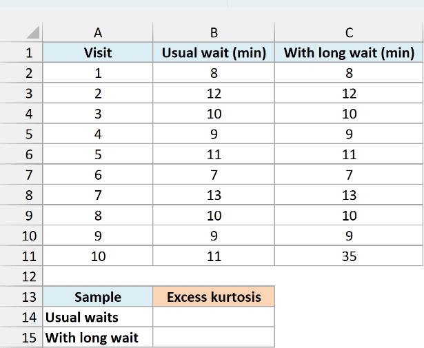
On the Example 1 sheet, enter this formula in cell B14 for the usual waiting times:
=KURT(B2:B11)
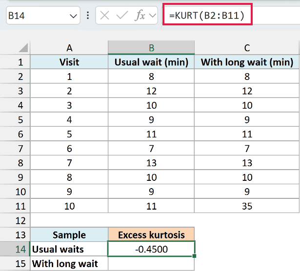
The formula uses the ten numbers in B2:B11 and returns -0.4500, displayed to four decimal places. KURT reduces the whole range to one number; it doesn’t return a separate result for each visit.
To understand that negative number, start with the reference point. A normal, bell-shaped distribution has an excess kurtosis of 0, while its ordinary kurtosis is 3.
KURT uses the excess convention and includes a sample-size adjustment. You don’t need to subtract 3 from its result.
Here’s how to read the signs:
| Result | Interpretation |
|---|---|
| Positive | Suggests heavier tails, with more influence from extreme observations, than the normal reference. |
| Negative | Suggests lighter tails than the normal reference. |
| Near zero | Is close to the normal reference for this measure, but doesn’t prove the data is normally distributed. |
The tails are the ends of a distribution, where values lie far from the center. Kurtosis is about those extremes, so it shouldn’t be read simply as the height of a chart’s peak.
Now compare the second sample. Its last wait is 35 minutes instead of 11 minutes, and all the other waits stay the same.
Enter this formula in cell B15:
=KURT(C2:C11)
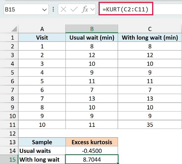
The result rises to 8.7044. The 35-minute wait sits much farther from the other observations, which shows how sensitive kurtosis is to an extreme value.
These ten-value samples make that effect easy to see. With a small sample, one observation can change the result a lot, so don’t treat the number as a reliable description of a much larger population by itself.
Important: KURT returns #DIV/0! when there are fewer than four numeric observations or all the numeric values are identical. Check both the number of values and whether they vary before interpreting an error.
The second case happens because identical values have zero standard deviation, and the kurtosis calculation divides by that measure of spread. Four identical numbers still won’t work.
Example 2: Handle Missing Values and Zeroes
A wait of zero minutes is a real observation. A missing wait is different, and KURT treats the two differently when you give it a cell range.
Below is a wait log containing numbers, a blank, text, and a TRUE value entered by mistake, and I want its excess kurtosis in cell B14.
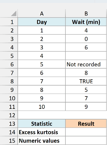
On the Example 2 sheet, enter this formula in cell B14:
=KURT(B2:B11)
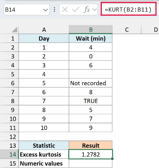
The result is 1.2782. The calculation uses 4, 0, 6, 8, 5, 7, and 9; it ignores the blank cell, the text “Not recorded”, and the logical value TRUE.
You can check the number of numeric observations with the COUNT function. Enter this formula in cell B15:
=COUNT(B2:B11)
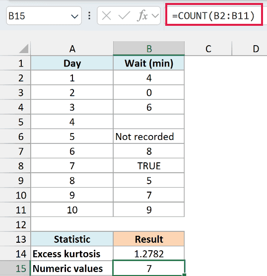
The result is 7, even though the log has ten rows. This count helps explain why a long-looking range can still contain too few numbers for KURT.
If an imported number is stored as text, KURT also ignores it in a range. Convert it to a real number before calculating, or that observation will be left out.
Important: Don’t replace missing observations with zero just to fill the gaps. KURT includes zero, so doing that changes the sample and can change the result.
KURT ignores logical values and numbers stored as text inside references or arrays. When you type a logical value or numeric text directly into its argument list, KURT counts that value instead.
Text typed directly into the argument list must be convertible to a number. A label such as “missing” entered there causes #VALUE! instead of being ignored.
Errors are different from text labels in cells. If the range contains an error such as #N/A, KURT returns that error, so fix the source cell before using the result.
Example 3: Calculate Kurtosis for One Group
Sometimes you only want the observations that belong to one category. The FILTER function can select those values before KURT calculates the result.
This example needs Excel for Microsoft 365, Excel 2024, Excel 2021, or Excel for the web because it uses FILTER.
Below is a visit log split into morning and evening sessions, and I want the selected session’s excess kurtosis in cell B16.
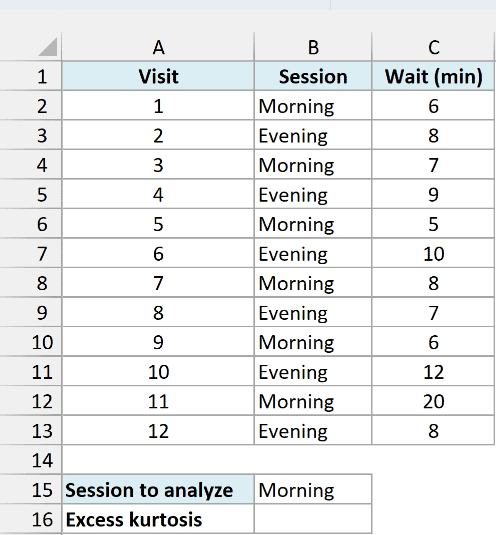
On the Example 3 sheet, cell B15 contains “Morning”. Enter this formula in cell B16:
=KURT(FILTER(C2:C13,B2:B13=B15))
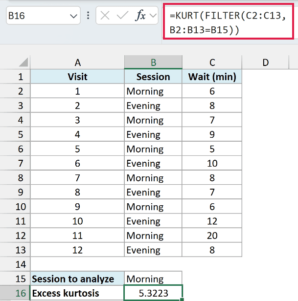
The result is 5.3223 for the six morning visits.
How this formula works:
B2:B13=B15checks which session labels match “Morning”.FILTER(C2:C13,B2:B13=B15)returns the matching waits: 6, 7, 5, 8, 6, and 20.- KURT calculates sample excess kurtosis from those six numbers and returns a single value.
The selected values pass directly from FILTER to KURT, so you don’t need a separate helper range on the sheet. The final formula still returns one cell, even though FILTER supplies several values internally.
Changing B15 to another session label makes the formula analyze that group. The two ranges must cover the same rows so each wait is tested against its own session label.
If the label doesn’t match any rows, this formula returns #CALC! because FILTER has no values to return. If it selects fewer than four numeric waits, or all selected waits are identical, KURT returns #DIV/0!.
Important: This example has a numeric wait in every row. FILTER can turn a matching blank source cell into zero, so resolve missing waits or explicitly exclude those rows before using this formula on an incomplete log.
In Excel 2019 or earlier, copy the matching observations into a separate range and apply KURT to that range. Merely hiding the other rows with a worksheet filter won’t exclude them from a normal KURT range calculation.
KURT gives you one useful measure of a sample’s shape. Check the underlying values alongside the result, especially when one unusually large or small observation could be driving it.
Other Excel Articles You May Also Like:
