

The STEYX function measures how far off your predictions are when you draw a straight line through paired data. Technically, it returns the standard error of the regression, which is the typical amount by which the actual values miss that line.
The result is in the same units as the values you’re predicting, so if you’re predicting sales in dollars, you get a dollar amount.
In this article, I’ll show you how to use it, how to read the result, and how to turn it into a rough prediction range.
Follow along with the example file
STEYX Function Examples.xlsx
STEYX Function Syntax
Here is the syntax of the STEYX function:
=STEYX(known_y's, known_x's)
- known_y’s – The values you want to predict, such as sales or price.
- known_x’s – The values you use to predict them, such as ad spend or mileage. It needs the same number of cells as known_y’s.
The order matters here. STEYX measures the error in known_y’s, so if you swap the two ranges, you get a different number that measures the error in the wrong values.
STEYX pairs the two ranges by position, so the first value in known_y’s goes with the first value in known_x’s, the second with the second, and so on.
If either value in a pair is a blank cell, text, or TRUE/FALSE, STEYX skips that whole pair. A zero is a real number, though, so a pair with a 0 stays in the calculation.
The STEYX function works in all current Excel versions, including Microsoft 365, Excel 2024, 2021, 2019, 2016, and Excel for Mac.
When to Use the STEYX Function
Use this function when you need to:
- Find the typical size of the miss when you predict values with a straight line
- Check how far off a forecast is likely to be, in the same units as your data
- Compare which of two factors predicts a result more accurately
- Build a rough range around a predicted value
- Get the prediction error for each group in a dataset
Let me show you five practical examples of how to use the STEYX function.
Example 1: Find the Standard Error of a Regression in Excel
Let’s start with a simple example.
Below is a log of weekly ad spend and sales for an online store, and I want to find the standard error of the sales predictions in cell F1.
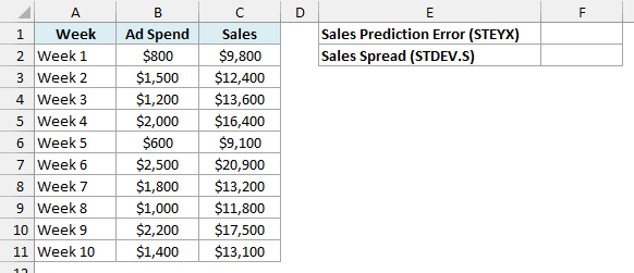
Here is the formula:
=STEYX(C2:C11,B2:B11)
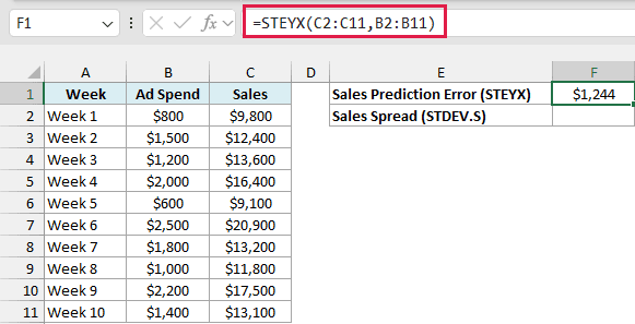
This gives $1,244. The sales in C2:C11 are the values I want to predict, so they go first, and the ad spend in B2:B11 goes second.
In plain words, if you use ad spend to predict a week’s sales with a straight line, the prediction will typically be off by about $1,244.
To judge whether $1,244 is big or small, compare it with how much sales swing on their own. Here is the formula with the STDEV.S function in cell F2:
=STDEV.S(C2:C11)
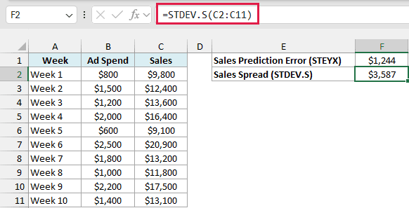
This gives $3,587, which is the typical miss if you predicted every week with the average sales. So knowing the ad spend brings the typical miss down from $3,587 to $1,244.
Important: If the two ranges don’t have the same number of cells, STEYX returns the #N/A error. A common cause is selecting the header in one range but not the other, as in =STEYX(C2:C11,B1:B11).
You’ll get the #DIV/0! error if you have fewer than three pairs of values, because STEYX divides by the number of pairs minus 2. You’ll also get it if every known_x’s value is the same, since there’s no slope to calculate.
Example 2: Compare Which Factor Predicts More Accurately
Now let’s use STEYX to compare two factors.
Below is a list of used cars with the mileage, age, and asking price of each, and I want to see which of the two predicts the price more accurately in cells G1 and G2.
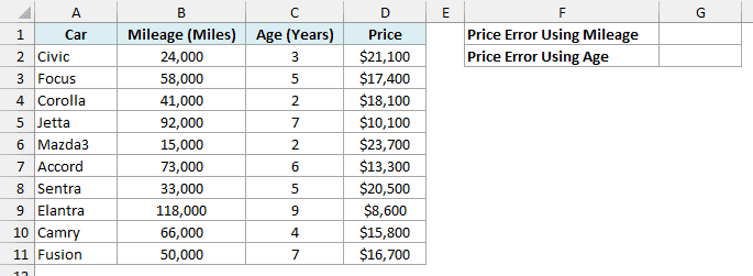
Here is the formula for the mileage in cell G1:
=STEYX(D2:D11,B2:B11)
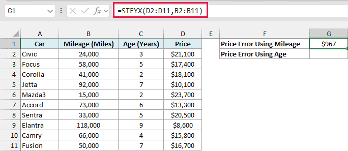
This gives $967, so a price predicted from mileage is typically off by about $967.
And here is the formula for the age in cell G2:
=STEYX(D2:D11,C2:C11)
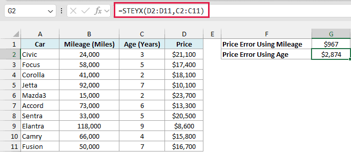
This gives $2,874, so a price predicted from age is typically off by almost three times as much.
Both formulas use the prices in D2:D11 as known_y’s, so both errors are in dollars and a smaller number means a better predictor. Only the second range changes.
So the mileage is a much better guide to the price than the age. That makes sense, since two cars of the same age can have very different mileage.
This comparison only works when the known_y’s are the same in both formulas. A STEYX for price and a STEYX for some other column are in different units, so you can’t compare them.
Example 3: Build a Rough Prediction Range Around a Forecast
Let’s step it up and use STEYX to put a range around a prediction.
Below is a list of lawn sizes in square feet with the minutes it took to mow each one, and I want to predict the mowing time for the lawn size in cell E1, along with a likely range.
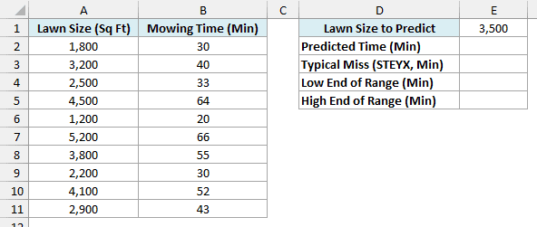
Here is the formula for the predicted time in cell E2:
=FORECAST.LINEAR(E1,B2:B11,A2:A11)
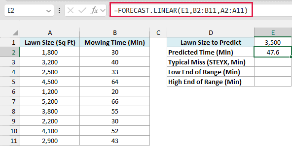
This gives 47.6 minutes for a 3,500 sq ft lawn. The FORECAST.LINEAR function predicts a value along the same straight line that STEYX measures the misses from.
In the formula, E1 is the lawn size to predict for, B2:B11 holds the mowing times, and A2:A11 holds the lawn sizes the line is drawn from.
Now here is the formula for the typical miss in cell E3:
=STEYX(B2:B11,A2:A11)
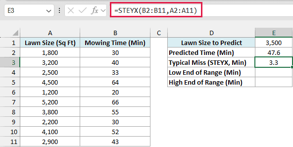
This gives 3.3 minutes. As a rule of thumb, about 95% of the points sit within two standard errors of the line when the misses are spread evenly around it, so two times this number makes a handy range.
Here is the formula for the low end of the range in cell E4:
=E2-2*E3
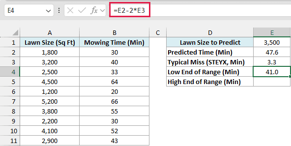
And here is the formula for the high end in cell E5:
=E2+2*E3
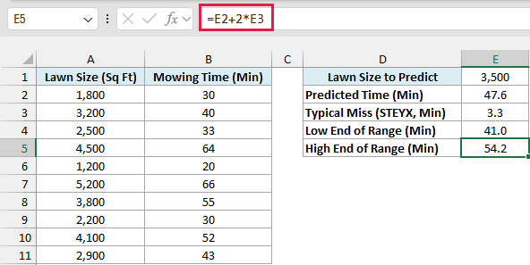
So a 3,500 sq ft lawn should take about 47.6 minutes, give or take 6.6 minutes, which is a range of 41.0 to 54.2 minutes. All 10 lawns in this data sit inside that band around the line.
This is only a rough range. With only 10 lawns, an exact 95% prediction interval would be a little wider, and it widens further for sizes far from the ones in your data.
Example 4: Check Where the STEYX Number Comes From
Let’s look under the hood to see exactly what STEYX measures.
Below is a price list of pizzas with the diameter and price of each, and I want to find the price the straight line predicts in column D and how far each actual price misses it in column E.
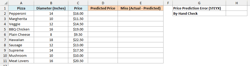
Here is the formula for the predicted price in cell D2:
=FORECAST.LINEAR(B2:B11,C2:C11,B2:B11)
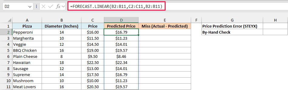
This spills the predicted price for all 10 pizzas into D2:D11. The first B2:B11 is the list of diameters to predict for, and the other two ranges are the prices and diameters the line is drawn from.
If you are using Excel 2019 or earlier, enter the below formula in cell D2 and then copy it down the range:
=FORECAST.LINEAR(B2,$C$2:$C$11,$B$2:$B$11)
Now here is the formula for the miss in cell E2:
=C2:C11-D2:D11
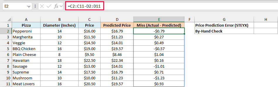
This subtracts the predicted price from the actual price for each pizza. A positive miss means the pizza costs more than the line predicts, and a negative miss means it costs less.
If you are using Excel 2019 or earlier, enter the below formula in cell E2 and then copy it down the range:
=C2-D2
Here is the STEYX formula in cell H1:
=STEYX(C2:C11,B2:B11)
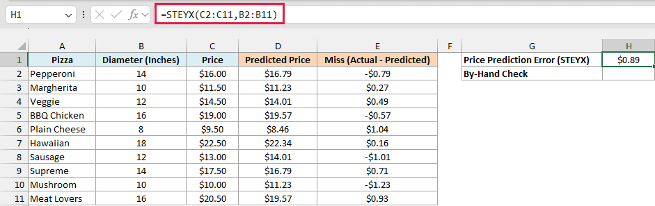
This gives $0.89. Now let’s build the same number by hand from the misses, with this formula in cell H2:
=SQRT(SUMSQ(E2:E11)/(COUNT(E2:E11)-2))
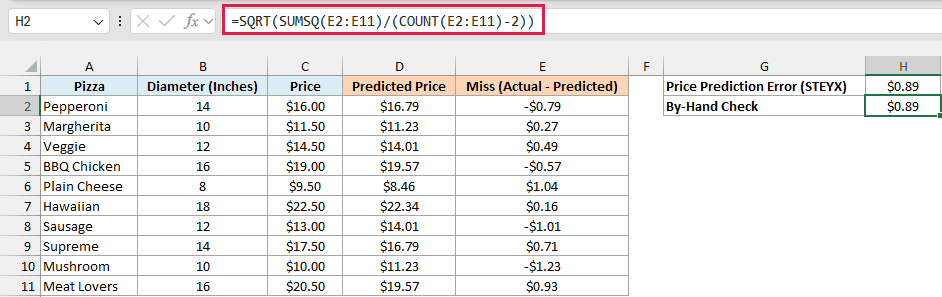
This gives $0.89 as well. How this formula works:
- The SUMSQ function squares each miss in E2:E11 and adds them up, so bigger misses count for more and the minus signs disappear.
- The sum of squares is divided by COUNT(E2:E11)-2, which is 10 pizzas minus 2. The line uses two numbers estimated from the data (the slope and the intercept), so two are taken off.
- The SQRT function takes the square root, which brings the result back to dollars.
So STEYX is a kind of average miss, with the big misses counting extra. The STDEV.S function divides by the count minus 1 instead of minus 2, so running it on the misses gives a slightly different number.
Example 5: Get the Standard Error for Each Group With One Formula
Finally, let’s get a separate standard error for each group.
Below is a log of sales calls with the region, the number of calls made, and the deals closed, and I want the standard error of the deals for each region in column F.
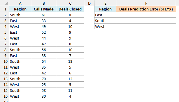
Here is the formula in cell F2:
=MAP(E2:E4,LAMBDA(region,STEYX(FILTER(C2:C16,A2:A16=region),FILTER(B2:B16,A2:A16=region))))
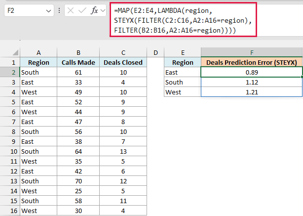
This spills three results into F2:F4. It gives 0.89 for East, 1.12 for South, and 1.21 for West.
How this formula works:
- MAP(E2:E4,…) goes through the region names in E2:E4 one at a time.
- LAMBDA(region,…) gives the current region name the name region.
- FILTER(C2:C16,A2:A16=region) keeps only the deals for that region, and FILTER(B2:B16,A2:A16=region) keeps only its calls.
- STEYX then finds the standard error for just those rows, and each result lands next to its region.
So in the East, the number of deals predicted from calls is typically off by 0.89 deals, while in the West it’s off by 1.21. East is the most predictable of the three.
Running STEYX on all 15 rows together gives 1.05. That number sits between the regional values, so it doesn’t show which region’s predictions are the most reliable.
The MAP function and the LAMBDA function are available in Excel 365 and Excel 2024. The FILTER function is available in Excel 365, 2024, and 2021.
If you are using Excel 2021 or earlier, enter the below formula in cell F2 (with Control + Shift + Enter in Excel 2019 or earlier) and then copy it down to F4:
=STEYX(IF($A$2:$A$16=E2,$C$2:$C$16,""),IF($A$2:$A$16=E2,$B$2:$B$16,""))
The two IF functions turn the deals and the calls from other regions into empty text, and STEYX skips text pairs, so only the matching region’s rows are used.
So these are five ways to use the STEYX function in Excel. STEYX gives you the size of the typical miss, and the INTERCEPT function and the SLOPE function give you the line itself.
If you want STEYX along with the other regression statistics, the LINEST function returns it as part of its full output.
I hope you found this article helpful.
Other Excel Articles You May Also Like:
