

The FORECAST.ETS.STAT function in Excel tells you how well a FORECAST.ETS forecast fits your past data. FORECAST.ETS predicts future values from the numbers you already have, and FORECAST.ETS.STAT returns one statistic about that forecast, such as the average size of its errors.
It works straight from your values and dates, so you don’t need a FORECAST.ETS formula in the sheet first.
These statistics are handy when you want to know whether you can trust a forecast, or which forecasting setup works better for your data.
In this article, I’ll explain what each of the eight statistics means and show you how to use them, from a simple error check to comparing several series at once.
Follow along with the example file
FORECAST.ETS.STAT Function Examples.xlsx
FORECAST.ETS.STAT Function Syntax
Here is the syntax of the FORECAST.ETS.STAT function:
=FORECAST.ETS.STAT(values, timeline, statistic_type, [seasonality], [data_completion], [aggregation])
- values – The historical numbers you want to forecast from.
- timeline – The dates (or period numbers) that go with those values. They need an even step, such as one day, one week, or one month.
- statistic_type – A number from 1 to 8 that picks which statistic you get back (the full list is below).
- [seasonality] – Optional. The length of the repeating pattern. Leave it out (or use 1) and Excel finds the pattern on its own, use 0 for no pattern, or enter a whole number such as 4, 7, or 12.
- [data_completion] – Optional. What to do with missing values. Leave it out (or use 1) to fill each gap with the average of its neighbors, or use 0 to treat gaps as zero.
- [aggregation] – Optional. How to combine values that share the same date. The default is 1 (AVERAGE). The others are 2 (COUNT), 3 (COUNTA), 4 (MAX), 5 (MEDIAN), 6 (MIN), and 7 (SUM).
Here is what each statistic_type number returns:
- 1 (Alpha) – How much weight the forecast gives to the latest values when it works out the level (the baseline value it builds on before adding any trend or seasonal pattern). It runs from 0 to 1, and a higher value means recent data counts for more.
- 2 (Beta) – The same kind of weight, but for the trend (how fast the numbers are rising or falling).
- 3 (Gamma) – The same kind of weight, but for the repeating seasonal pattern.
- 4 (MASE) – Mean absolute scaled error. It compares the forecast’s error with the error of a naive forecast, which simply guesses that each value will be the same as the one before. A value below 1 means the forecast did better than that naive guess.
- 5 (SMAPE) – Symmetric mean absolute percentage error. It’s the error as a percentage, which lets you compare data of very different sizes.
- 6 (MAE) – Mean absolute error. It’s the average size of a miss, in the same units as your data.
- 7 (RMSE) – Root mean squared error. It’s also in your data’s units, but it gives big misses more weight than MAE does.
- 8 (Step size) – The step Excel detected between the points in your timeline.
The error statistics (4 to 7) are worked out from your historical data. Excel compares the values the forecast predicts for your past periods with the actual values, and each gap between the two is a miss.
So these statistics tell you how well the forecast fits the past, which is a good guide but not a guarantee of how it will do in the future.
The statistic_type has to be a whole number from 1 to 8. Anything else, such as 0, 9, or 2.5, returns the #NUM! error.
The FORECAST.ETS.STAT function works in Microsoft 365, Excel 2024, 2021, 2019, and 2016 on Windows, and in Microsoft 365, 2024, and 2021 on Mac. It is not available in Excel for the web or in the Excel mobile apps.
When to Use the FORECAST.ETS.STAT Function
Use this function when you need to:
- Find out how far off a forecast is on average, in the same units as your data
- Check whether a forecast does better than simply repeating the last value
- Compare seasonality settings and keep the one with the smallest error
- Compare how predictable different items are, even when their sizes are very different
- See the smoothing weights and the timeline step that Excel used
Let me show you a few practical examples of how to use the FORECAST.ETS.STAT function in Excel.
Example 1: Find the Average Forecast Miss (MAE)
Let’s start with a simple example.
Below I have the number of visitors at a zoo for each quarter from 2023 to 2025, and I want to find how far off the forecast is on average in cell E2.
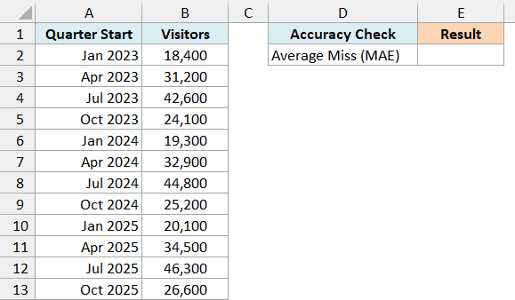
Here is the formula:
=FORECAST.ETS.STAT(B2:B13,A2:A13,6)
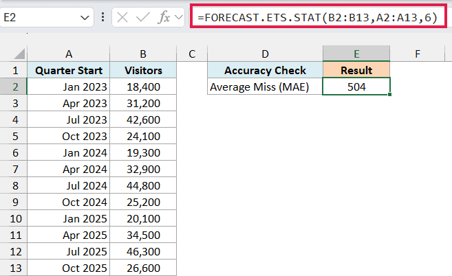
B2:B13 has the visitor counts, A2:A13 has the quarter dates, and 6 asks for the MAE (mean absolute error). The formula returns 504, so on average the forecast misses the actual count by about 504 visitors.
MAE is in the same units as your data, which makes it easy to judge. The zoo gets between 18,400 and 46,300 visitors a quarter, so a miss of about 504 is small.
I left out the three optional arguments, so Excel uses their defaults. It looks for a repeating pattern on its own, and here it picks up the four-quarter cycle of busy summers and quiet winters.
Example 2: Get All Eight FORECAST.ETS.STAT Statistics at Once
Now let’s pull out every statistic with one formula.
Below I have the number of cars washed each day at a car wash over four weeks, and I want to get all eight statistics for this data in column F.
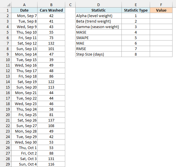
Here is the formula:
=FORECAST.ETS.STAT(B2:B29,A2:A29,E2:E9)
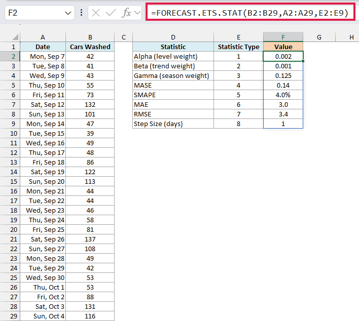
This time the statistic_type argument is the range E2:E9, which holds the numbers 1 to 8. So FORECAST.ETS.STAT returns one result for each number and spills all eight into F2:F9.
Here’s how to read the results:
- Alpha (0.002) and Beta (0.001) are both close to zero. So the forecast barely adjusts its level and trend for the latest days, and leans on the full four weeks instead.
- Gamma (0.125) is the only weight doing real work here. It lets the weekly pattern (quiet weekdays, busy weekends) update a little from recent weeks.
- MASE (0.14) is well below 1, so the forecast does much better than a naive one.
- SMAPE (4.0%) says the forecast is off by about 4% on average.
- MAE (3.0) and RMSE (3.4) say a typical miss is about 3 cars a day.
- Step size (1) means Excel found one day between the dates.
FORECAST.ETS.STAT returns every result as a plain decimal, so SMAPE comes back as 0.0395. I formatted that cell as a percentage to show it as 4.0%.
For a date timeline, the step size is counted in days. So weekly dates return 7, monthly dates on the 1st return 31, and quarterly dates return 90.
Spilling formulas like this one need Excel 2021 or Microsoft 365. If you are using Excel 2019 or 2016, enter the below formula in cell F2 and then copy it down to F9:
=FORECAST.ETS.STAT($B$2:$B$29,$A$2:$A$29,E2)
Example 3: Check If the Forecast Beats a Simple Guess (MASE)
Here’s another practical scenario.
Below I have the number of pets adopted from an animal shelter each month in 2025, and I want to get the MASE in cell E2 and a plain verdict in cell E3.
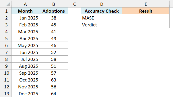
Here is the formula for the MASE:
=FORECAST.ETS.STAT(B2:B13,A2:A13,4)
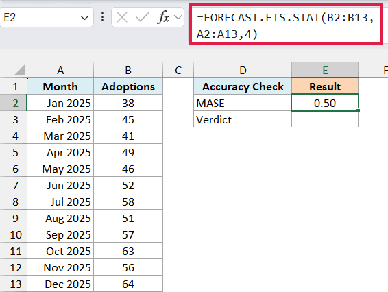
As you saw in the syntax section, MASE compares the forecast’s error with the error of a naive forecast. Here, that naive forecast just guesses that each month will be the same as the month before.
The standard way to read it is simple. Below 1, the forecast beats that naive guess, and above 1, the naive guess does better.
Here the result is 0.50, so the forecast’s error is about half of what the naive guess would give.
Now, here is the formula for the verdict:
=IF(E2<1,"Beats a naive guess","Naive guess does better")
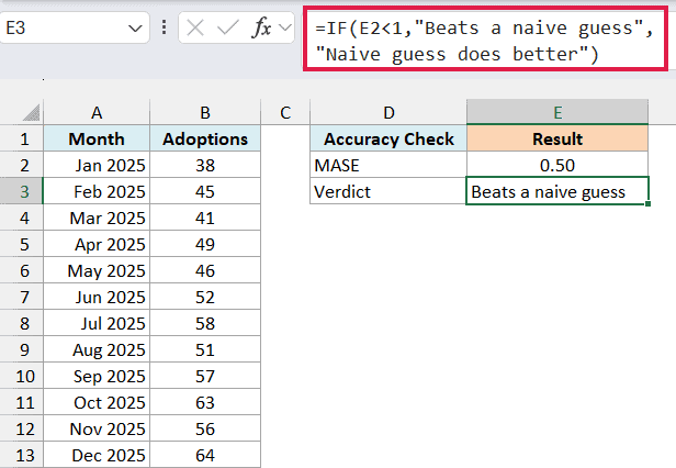
This IF formula checks whether the MASE in E2 is below 1 and returns “Beats a naive guess”. It’s a useful way to label results when you check many products or series at once.
If you ever get a MASE above 1, the simple “same as last month” guess would have been closer. So for that data, the ETS forecast isn’t adding much.
Example 4: Compare Seasonality Settings to Pick the Best One
Now let’s look at something more interesting.
Below I have a household’s monthly water use for 2024 and 2025, and I want to compare the forecast error for three seasonality settings in column F.
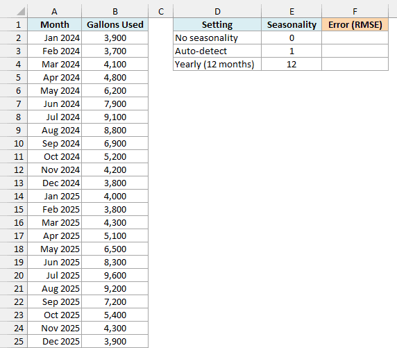
Here is the formula:
=FORECAST.ETS.STAT(B2:B25,A2:A25,7,E2:E4)
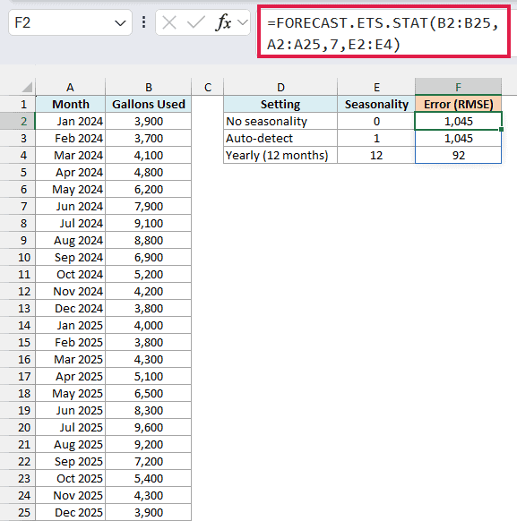
The 7 asks for the RMSE, and the seasonality argument is the range E2:E4 (0, 1, and 12). So the formula works out the error once for each setting and spills the three results into F2:F4.
RMSE is in gallons, just like the data. It squares each miss before averaging, so a few large misses push it up more than they would push up the MAE.
With no seasonality (0), the forecast misses by about 1,045 gallons. Auto-detect (1) gives the exact same number, because Excel’s automatic check didn’t find a repeating pattern in this data.
You can confirm that with the FORECAST.ETS.SEASONALITY function, which reports the pattern length Excel detects. On this data, it returns 0.
But there clearly is a pattern here, since water use peaks every summer and drops every winter. Telling Excel that the pattern repeats every 12 months cuts the error to 92 gallons.
So auto-detect can miss a pattern you can see in your data. That’s why it’s worth testing the settings that make sense and keeping the one with the smallest error.
Then use that same setting in your FORECAST.ETS formula.
If you are using Excel 2019 or 2016, enter the below formula in cell F2 and then copy it down to F4:
=FORECAST.ETS.STAT($B$2:$B$25,$A$2:$A$25,7,E2)
Example 5: See How Missing Weeks Change the Error
Real-world logs often have gaps, and the data_completion argument decides how they’re handled.
Below I have a household’s weekly grocery bill for 12 weeks, with two weeks that were never logged, and I want to compare the average miss with the gaps filled in (cell E2) and with the gaps counted as zero (cell E3).
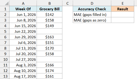
Here is the formula that fills in the gaps:
=FORECAST.ETS.STAT(B2:B13,A2:A13,6)
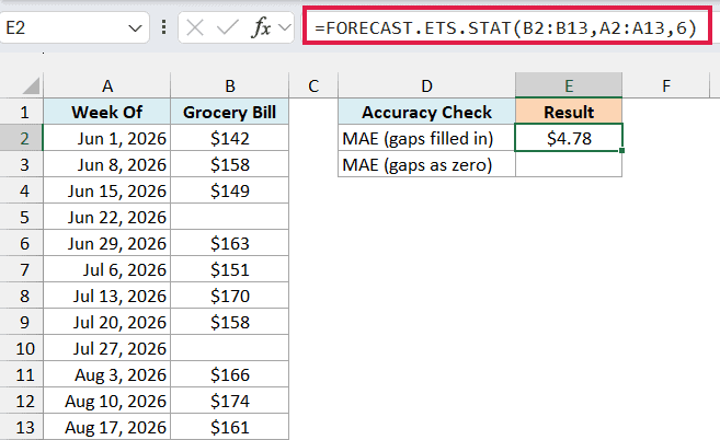
With data_completion left out, Excel fills each blank week with the average of the weeks on either side. The forecast then misses by $4.78 on average, which is small for bills of $142 to $174.
Now, here is the formula that counts the gaps as zero:
=FORECAST.ETS.STAT(B2:B13,A2:A13,6,,0)
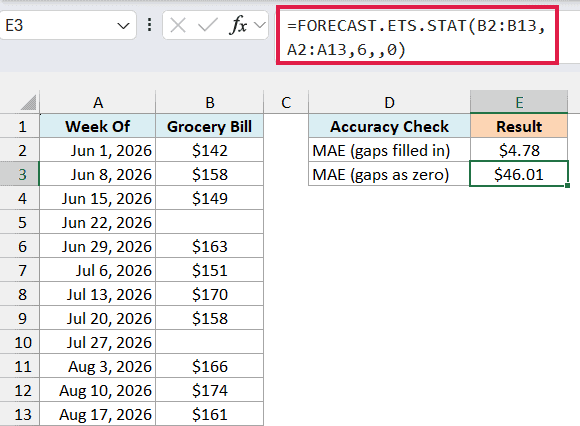
The 0 in the data_completion argument turns the two blank weeks into $0 bills. The empty spot between the commas skips the seasonality argument, so it keeps its default.
The forecast can’t predict a sudden $0 week, so the average miss jumps to $46.01. So use 0 only when a blank really means zero, and leave data_completion out when a value just wasn’t written down.
Microsoft says FORECAST.ETS.STAT can handle up to 30% of the values missing. But the fewer the gaps, the more you can trust the statistics.
Example 6: Compare Which Series Is Easiest to Forecast (SMAPE)
Let’s step it up with a more advanced use case.
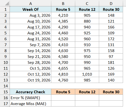
Below I have the weekly riders on three bus routes for 12 weeks, and I want to get each route’s SMAPE in row 16 and its MAE in row 17.
Here is the formula for the SMAPE:
=BYCOL(B2:D13,LAMBDA(r,FORECAST.ETS.STAT(r,A2:A13,5)))
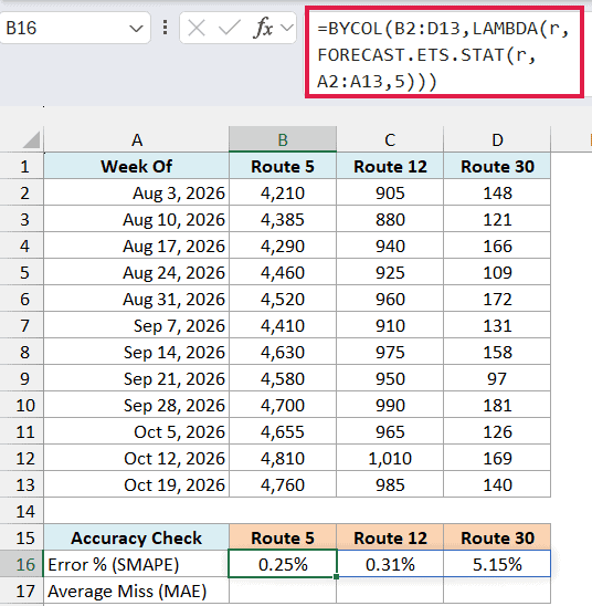
How this formula works:
- The BYCOL function takes the riders in B2:D13 and hands them to the LAMBDA one column (one route) at a time.
- Inside the LAMBDA, r stands for that route’s column. FORECAST.ETS.STAT(r,A2:A13,5) returns its SMAPE, using the same week dates for every route.
- BYCOL puts the three results side by side, so they spill into B16:D16.
Route 30 has the highest SMAPE (5.15%), while Routes 5 and 12 stay below a third of a percent. So Route 30 is by far the hardest to forecast.
Now, here is the formula for the MAE:
=BYCOL(B2:D13,LAMBDA(r,FORECAST.ETS.STAT(r,A2:A13,6)))
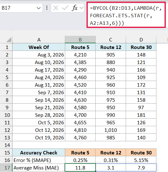
This is the same formula with 6 (MAE) instead of 5. And here, Route 5 has the biggest miss (11.8 riders), while Route 30 sits at 7.9.
That’s because MAE is in riders, and Route 5 carries over 4,000 riders a week. A miss of 12 riders on a route that big is tiny, while a miss of 8 riders on a route with about 140 is not.
So use MAE or RMSE when you want the error of one series in real units, and SMAPE when you’re comparing series of different sizes.
The BYCOL and LAMBDA functions need Microsoft 365 or Excel 2024. If you are using an older version, enter the below formula in cell B16 and then copy it across to D16:
=FORECAST.ETS.STAT(B2:B13,$A$2:$A$13,5)
Use the same formula with 6 instead of 5 in row 17 to get the MAE.
In this article, I showed you how to use the FORECAST.ETS.STAT function to find a forecast’s average miss, pull all eight statistics at once, check a forecast against a naive guess, compare seasonality settings, handle missing values, and compare series of different sizes.
To make the forecast itself, use the FORECAST.ETS function. It takes the same values, timeline, and optional settings, plus the date you want a forecast for.
I hope you found this article helpful.
Other Excel Articles You May Also Like:
