
The Chi-Square test lets you figure out if two things in your data are actually related.
Maybe you ran a survey and want to know if gender affects car color preference. Or you’re looking at student results and wondering whether the teaching method makes a difference in pass rates.
It works with any data where you’re comparing categories against categories. In this article, I’ll show you how to calculate Chi-Square in Excel.
➡️ Click here to download the example file and follow along
Using the CHISQ.TEST Function (Recommended)
The CHISQ.TEST function is the quickest way to calculate the Chi-Square value in Excel.
You give it two ranges (actual values and expected values), and it tells you whether the relationship in your data is real or just random.
Before we use this function, we need our data set up properly.
Let’s say I surveyed 200 customers (both Males and Females) and recorded their car color preference (three choices: Red, Blue, and White).
I organized the results into a table where the rows are the two genders and the columns are the three colors. Each cell shows how many customers picked that combination.
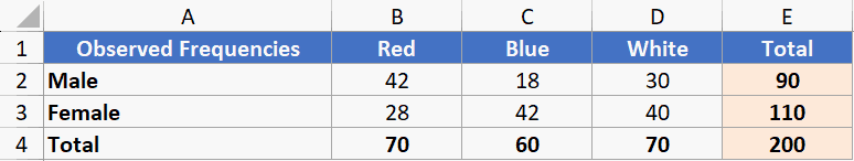
This type of table is called a contingency table.
Now, the CHISQ.TEST function needs two things:
- Observed data (what you actually collected) and
- something called Expected frequencies.
Imagine gender had zero influence on which color people chose. You’d expect Males and Females to pick each color at roughly the same rate, proportional to their group sizes.
For example, if there are 100 males and 100 females, they would pick each colored car the same number of times.
You can calculate exactly what those “no influence” numbers would look like.
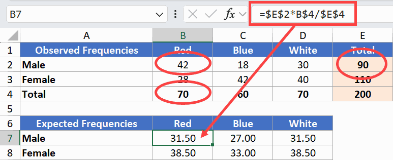
The formula for each cell is:
(Row Total × Column Total) / Grand TotalFor example, the Male row total is 90, the Red column total is 70, and the grand total is 200. So the expected value for Male + Red is (90 × 70) / 200 = 31.5.
I’ve calculated the expected values for every cell using this same formula.
Now, here is the formula that gives us the p-value for the Chi-Square test:
=CHISQ.TEST(B2:D3,B7:D8)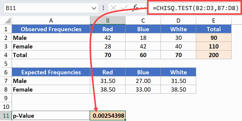
How does this formula work?
CHISQ.TEST takes two arguments. The first (B2:D3) is your observed data. The second (B7:D8) is your expected frequencies.
It returns a p-value, which is the probability that the pattern in your data is just random chance.
Here, the p-value is approximately 0.0025. That’s well below 0.05, which means gender and car color preference are actually related in this data.
If the p-value had been greater than 0.05, the differences would likely be random.
Calculating Chi-Square Manually Using Formulas
Here’s another way to do this. Instead of relying on one function, you can build the calculation step by step.
This is useful when you need the actual Chi-Square statistic for a report, or when you want to see which cells are driving the result.
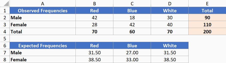
Below, I have the same observed and expected frequency tables from the previous method.
Here is the formula for the first cell:
=(B2-B7)^2/B7Copy it across all six cells in the table.
And if you’re using Excel that has dynamic arrays, you can also use:
=(B2:D3-B7:D8)^2/B7:D8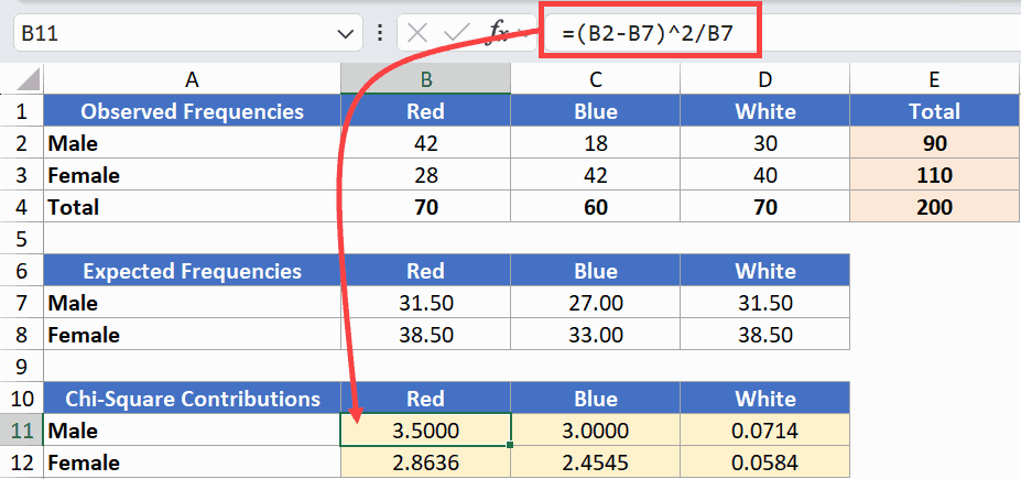
How does this formula work?
This measures how far each observed value deviates from what was expected.
You square the difference so that negatives and positives don’t cancel each other out. Dividing by the expected value keeps it proportional.
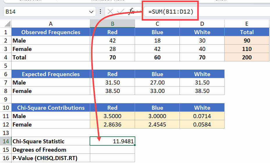
Next, add up all six values to get the Chi-Square statistic:
=SUM(B11:D12)In this example, it comes out to approximately 11.95.
Now you need the degrees of freedom.
The formula for this is (number of rows – 1) × (number of columns – 1).
So, I have used the following formula to calculate the degrees of freedom:
=(ROWS(B2:B3)-1)*(COLUMNS(B2:D2)-1)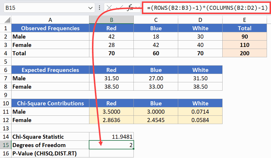
Finally, convert the Chi-Square statistic into a p-value:
=CHISQ.DIST.RT(B16,2)CHISQ.DIST.RT takes the statistic and the degrees of freedom and returns the p-value.
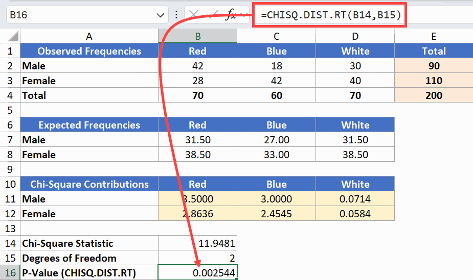
Same result as Method 1. But now you also have the Chi-Square statistic itself (11.95), and you can see which cells contributed the most.
Alternative: Using a Critical Value instead of a p-value
There is another manual way to calculate the chi-square value in Excel.
Instead of checking the p-value, you compare your Chi-Square statistic against a threshold called the critical value.
To get the critical value, use the below CHISQ.INV.RT formula:
=CHISQ.INV.RT(level of significance , degrees of freedom)
So in our case, this is the formula I would use.
=CHISQ.INV.RT(0.05,B15)The first argument is your significance level (0.05), and the second is the degrees of freedom. This returns approximately 5.99.
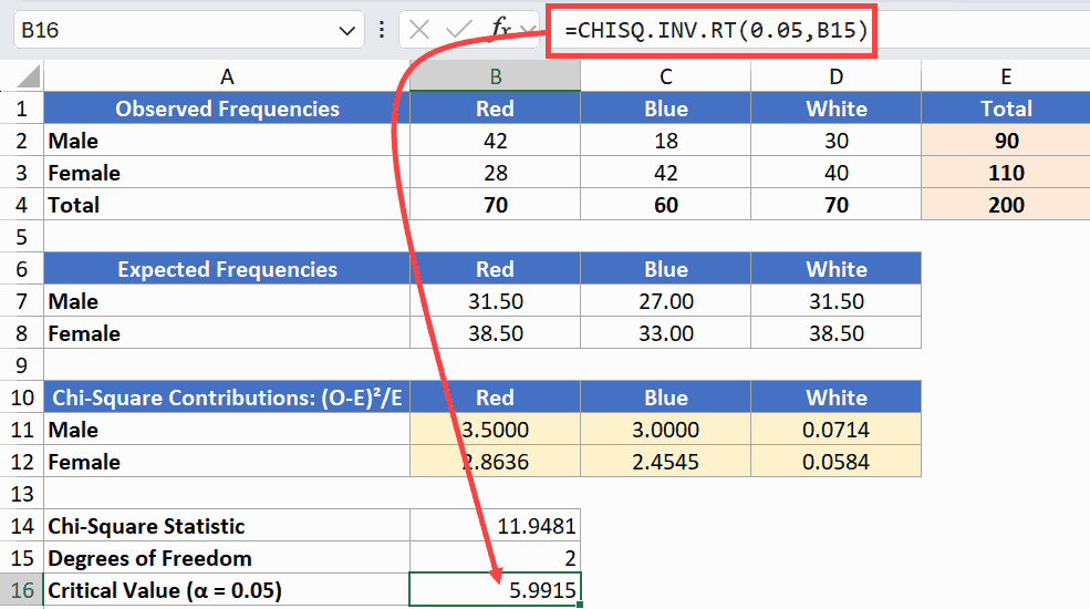
Since 11.95 (which is our chi-square statistic) is greater than 5.99 (which is the critical value), you reject the null hypothesis.
Same conclusion as before.
If your statistic had been less than 5.99, the relationship would not be significant.
Things to Keep in Mind
- Every cell in your expected frequency table should be at least 5. If any cell falls below that, the test may not give reliable results.
- Chi-Square works with frequency counts, not percentages or proportions. Make sure your data has actual counts (like 42 customers), not percentage values.
- The observed and expected ranges in CHISQ.TEST must be the same size. If they don’t match, the formula will return an error.
- A significant result tells you a relationship exists, but not how strong it is. Looking at the individual (O-E)²/E values can help you spot which cells are driving the result.
- CHISQ.TEST was introduced in Excel 2010. If you’re on an older version, use CHITEST instead.
- A p-value less than 0.05 means the result is statistically significant. Greater than 0.05 means the differences could be due to chance.
In this article, I showed you how to calculate Chi-Square in Excel using the CHISQ.TEST function and the manual formula approach.
I hope you found this article helpful.
Other Excel articles you may also like:


