

The AMORDEGRC function calculates depreciation for a specified accounting period using an older French declining-balance method. It applies a multiplier based on an asset’s useful life and adjusts the first period for the purchase date.
Microsoft has deprecated AMORDEGRC because the French depreciation method has changed. The function remains available for older workbooks, so the examples below focus on understanding and checking those calculations.
I’ll show you how to calculate the first period, inspect a period-by-period schedule, and see how the day-count basis and annual rate affect the result.
Follow along with the example file
AMORDEGRC Function Examples.xlsx
AMORDEGRC Function Syntax
Here is the syntax of the AMORDEGRC function:
=AMORDEGRC(cost, date_purchased, first_period, salvage, period, rate, [basis])
- cost: The asset’s original purchase cost.
- date_purchased: The date the asset was bought. Supply a real Excel date.
- first_period: The end date of the first accounting period, not its starting date.
- salvage: The estimated value left at the end of the asset’s life.
- period: The accounting period to calculate. Use 0 for the first partial period, then 1, 2, and so on for later annual periods.
- rate: The ordinary annual depreciation rate, entered as a percentage or decimal. AMORDEGRC applies its depreciation multiplier internally.
- basis: Optional. The day-count convention used for the first period: 0 for US 30/360, 1 for actual/actual, 3 for actual/365, or 4 for European 30/360.
Omitting basis uses 0, the US/NASD 30/360 convention. It doesn’t use the convention set by your computer’s region, so supply this argument when matching an existing workbook that uses another basis.
Enter a 20% annual rate as 20% or 0.2, not 20. The rate also determines the assumed life: 20% corresponds to five years because 1 divided by 0.2 is 5.
AMORDEGRC is available in Excel for Microsoft 365, 2024, 2021, 2019, and 2016. The spilling examples below need Microsoft 365, 2024, or 2021; copy-down alternatives are included for older Excel.
When to Use the AMORDEGRC Function
Use this function when you need to:
- Reproduce an AMORDEGRC calculation in an older workbook.
- Check the first-period amount for an asset purchased during the year.
- Investigate differences caused by period numbers, day-count conventions, or rates.
These are legacy-workbook checks. AMORDEGRC is no longer recommended for a new depreciation model.
Let’s start with one asset and one accounting period.
Example 1: Calculate First-Period Depreciation
Below are the inputs for a photocopier purchased during the year, and I want to calculate its first-period depreciation in cell B10.
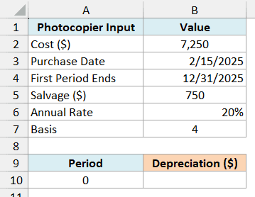
Enter this formula in cell B10:
=AMORDEGRC(B2,B3,B4,B5,A10,B6,B7)
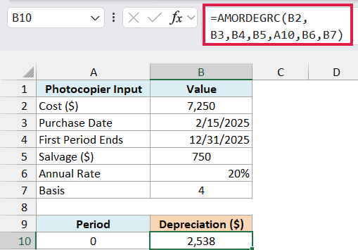
The formula returns $2,538 for the photocopier bought on February 15, 2025, with a first period ending December 31, 2025. The 0 in A10 tells AMORDEGRC to calculate that initial partial period.
The 20% rate implies a five-year life, for which AMORDEGRC uses a multiplier of 2. That gives an effective rate of 40%, and basis 4 counts this first period as 315 out of 360 days.
So the calculation is $7,250 multiplied by 40%, then by 315/360. That gives $2,537.50, which AMORDEGRC rounds to the whole-unit result of $2,538.
The dates in the example are real Excel dates, displayed in month/day/year format. If your inputs are text, Excel may interpret them differently under another regional setting, so convert them to dates or build them with the DATE function.
Make sure first_period is the period’s end date and isn’t earlier than the purchase date. Also keep period 0 distinct from period 1: period 1 asks for the following annual period, not the initial partial period.
Example 2: Inspect a Depreciation Schedule
For an older workbook, it helps to see what AMORDEGRC returns across several periods instead of checking just the first amount.
Below are the inputs for a workshop cutter and a list of periods from 0 to 5, and I want to return the depreciation for each period in column B.
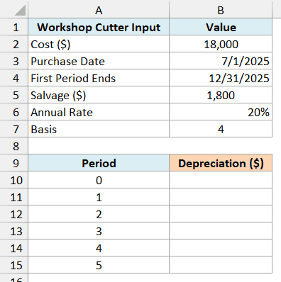
Enter this formula in cell B10:
=AMORDEGRC(B2,B3,B4,B5,A10:A15+0,B6,B7)
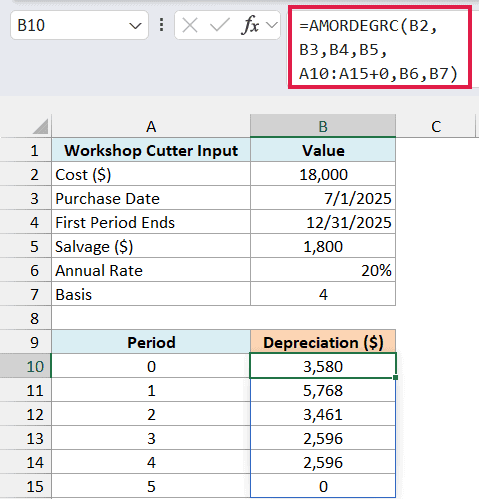
The formula returns 3,580, 5,768, 3,461, 2,596, 2,596, and 0, spilling the six amounts down column B. Each amount corresponds to the period beside it.
The +0 is needed here because AMORDEGRC doesn’t accept the multi-cell reference directly. Adding zero turns the numeric range into an array of values that the function can process; using the bare range returned #VALUE! in Excel testing.
This conversion doesn’t ignore blanks. A blank period becomes 0 and repeats the first-period calculation, so keep the period list complete and leave the output cells below B10 empty for the spill.
Period 0 covers the purchase on July 1, 2025, through December 31, 2025. Period 1 is the next full annual period, so its $5,768 amount can be larger than the initial $3,580 partial-period amount.
For period 1, Excel applies 40% to the $14,420 left after period 0, giving $5,768. The later amounts also reflect the function’s rounding and special treatment of the final periods, so they don’t all follow one repeated percentage calculation.
Important: These native results total $18,001, although cost minus salvage is $16,200. Don’t assume AMORDEGRC will stop at the salvage value; check the complete schedule when reviewing a legacy workbook.
If you are using Excel 2019 or earlier, enter the below formula in cell B10 and copy it down through B15:
=AMORDEGRC($B$2,$B$3,$B$4,$B$5,A10,$B$6,$B$7)
The dollar signs create absolute references that keep the asset inputs fixed while A10 changes to A11, A12, and so on. This returns the same amounts one row at a time.
Follow along with the example file
AMORDEGRC Function Examples.xlsx
Example 3: Compare Day-Count Bases
Two formulas can use the same asset and rate but return different first-period amounts because they count the partial year differently.
Below are the photocopier inputs from the first example and four basis codes, and I want to compare their first-period depreciation in column B.
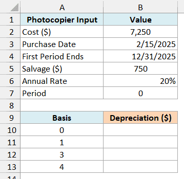
Enter this formula in cell B10:
=AMORDEGRC(B2,B3,B4,B5,B7,B6,A10:A13+0)
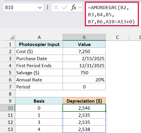
Here, the period stays fixed at 0 in B7, while the last argument changes for each basis code. The +0 uses the same numeric-array conversion as the previous example.
The results are:
- 0, US/NASD 30/360: $2,546.
- 1, actual/actual: $2,535.
- 3, actual/365: $2,535.
- 4, European 30/360: $2,538.
Bases 1 and 3 agree for these dates because 2025 has 365 days. Bases 0 and 4 both use a 360-day year, but their rules for adjusting month-end dates differ, which changes the amount here.
Important: AMORDEGRC doesn’t support basis 2, even though some other financial functions do. Using 2 returns #NUM!, so match the original workbook’s valid basis rather than choosing it as an actual/360 option.
If you are using Excel 2019 or earlier, enter the below formula in cell B10 and copy it down through B13:
=AMORDEGRC($B$2,$B$3,$B$4,$B$5,$B$7,$B$6,A10)
Example 4: Understand the Rate Multiplier
A lower annual rate doesn’t always produce a lower AMORDEGRC result. Changing the rate also changes the assumed life, which can put the asset into a different multiplier category.
Below are the inputs for legacy equipment and three annual rates, and I want to compare the first-period depreciation in column B.
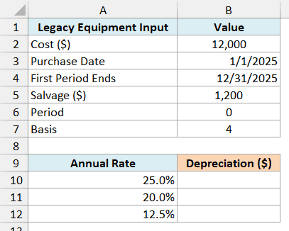
Enter this formula in cell B10:
=AMORDEGRC(B2,B3,B4,B5,B6,A10:A12+0,B7)
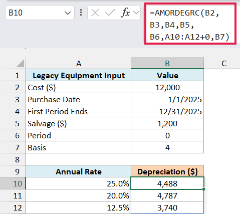
The formula returns $4,488 at 25%, $4,787 at 20%, and $3,740 at 12.5%. The asset cost, dates, salvage value, period, and basis remain the same in all three calculations.
Here is why the amounts change:
- A 25% rate implies a four-year life. The legacy coefficient is 1.5, so the effective rate is 37.5%.
- A 20% rate implies a five-year life. The coefficient is 2, so the effective rate is 40%.
- A 12.5% rate implies an eight-year life. The coefficient is 2.5, so the effective rate is 31.25%.
That explains why 20% produces more depreciation than 25% in this example. The coefficient raises its effective rate to 40%, compared with 37.5% for the 25% input.
The dates run from January 1 to December 31, 2025. Under basis 4, that interval is 359/360 of a year, so the first-period amounts are slightly below the full-year figures of $4,500, $4,800, and $3,750 before whole-unit rounding.
Important: Pass the ordinary annual rate to AMORDEGRC. Don’t multiply it by the coefficient beforehand, because the function selects and applies its coefficient itself.
If you are using Excel 2019 or earlier, enter the below formula in cell B10 and copy it down through B12:
=AMORDEGRC($B$2,$B$3,$B$4,$B$5,$B$6,A10,$B$7)
These examples show how to check AMORDEGRC’s first period, later periods, day-count basis, and rate multiplier in an older workbook. I hope you found this Excel tutorial useful.
Other Excel Articles You May Also Like:
