SLN Function in Excel

The SLN function in Excel calculates straight-line depreciation, which is the amount an asset loses in value each period when that loss is spread evenly over its life.

You give it the cost, the value at the end, and the life, and it returns one fixed amount per period.

It’s the simplest and most common way to depreciate an asset, and it suits things that wear out at a steady pace, like vehicles, furniture, and office equipment.

The examples start with one asset and move on to whole asset lists, monthly figures, a book value schedule, assets bought partway through the year, and totals by department.

SLN Function Syntax

Here is the syntax of the SLN function:

=SLN(cost,salvage,life)

• cost – the price you paid for the asset.
• salvage – what you expect the asset to be worth at the end of its useful life (sometimes called the residual value). Use 0 if you expect it to be worth nothing.
• life – the number of periods over which the asset is depreciated (its useful life).

All three arguments are required. SLN simply subtracts the salvage value from the cost and divides the result by the life, so you get the same amount for every period.

The period is whatever unit you use for life. Enter the life in years and SLN returns yearly depreciation; enter it in months and you get monthly depreciation.

If life is 0 or the cell is empty, SLN returns the #DIV/0! error, because it ends up dividing by zero.

And if the salvage value is higher than the cost, you get a negative result, which is usually a sign of a typo in the inputs.

The SLN function works in Excel 365, 2024, 2021, 2019, 2016, and Excel for Mac.

When to Use the SLN Function

Use this function when you need to:

• Work out how much an asset depreciates each year
• Calculate depreciation for a whole list of assets at once
• Get monthly depreciation for monthly reports
• Build a schedule that shows an asset’s book value year by year
• Total up depreciation expense for a group of assets

Let me show you a few practical examples of how to use the SLN function.

Example 1: Calculate Yearly Straight-Line Depreciation

Let’s start with a simple example.

Below are the details of a delivery van a bakery bought, and I want to get its yearly depreciation in cell B6.

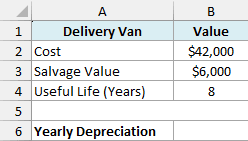
Here is the formula:

=SLN(B2,B3,B4)

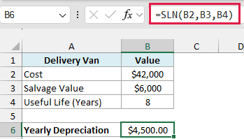
The formula returns $4,500.00, which is how much the van loses in value each year.

Behind the scenes, SLN takes the cost of $42,000, subtracts the salvage value of $6,000, and spreads the remaining $36,000 evenly over 8 years.

So you would get the same answer with =(B2-B3)/B4, but SLN makes it clear at a glance that this is a depreciation calculation.

Since the formula points to cells, you can change the cost, salvage value, or life, and the depreciation updates right away.

Example 2: Straight-Line Depreciation for a List of Assets

In real life, you usually have more than one asset to depreciate.

Below is a list of equipment a café owns, with the cost, salvage value, and useful life of each item, and I want to get the yearly depreciation for all of them in column E.

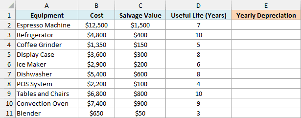
Here is the formula:

=SLN(B2:B11,C2:C11,D2:D11)

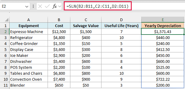
You enter this one formula in cell E2, and it spills the yearly depreciation for all ten items down to E11.

Since each argument is a range, SLN works through the rows one by one, using the cost, salvage value, and life from the same row. For example, the espresso machine loses ($12,500 – $1,500) / 7 = $1,571.43 a year.

The cells below E2 need to be empty for the results to spill. If something is in the way, you’ll see a #SPILL! error instead.

If you are using Excel 2019 or earlier, enter the below formula in cell E2 and then copy it down the range:

=SLN(B2,C2,D2)

Example 3: Calculate Monthly Depreciation

Many businesses report their numbers every month, so they need depreciation per month and not per year.

Below is a list of gym equipment with the useful life in years, and I want to get the monthly depreciation for each item in column E.

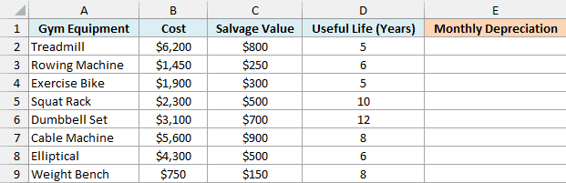
Here is the formula:

=SLN(B2:B9,C2:C9,D2:D9*12)

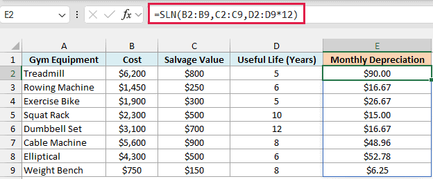
The trick here is in the third argument. D2:D9*12 converts the useful life from years to months, so SLN spreads the loss in value over months and returns a monthly amount.

For the treadmill, that’s ($6,200 – $800) / 60 months = $90.00 per month.

You’d get exactly the same result with =SLN(B2:B9,C2:C9,D2:D9)/12, which takes the yearly figure and divides it by 12. Use whichever reads more naturally to you.

If you are using Excel 2019 or earlier, enter the below formula in cell E2 and then copy it down the range:

=SLN(B2,C2,D2*12)

Important: If you forget the *12, SLN still uses the life in years and returns yearly figures. They would sit under the Monthly Depreciation header looking perfectly normal, so double-check the unit of the life.

Example 4: Create a Book Value Schedule With SLN

The book value is what an asset is still worth on your books after the depreciation so far. A schedule that shows it for every year is a common thing to build next to SLN.

Below are the details of a company car, along with the years of its useful life in column D, and I want to get the book value at the end of each year in column E.

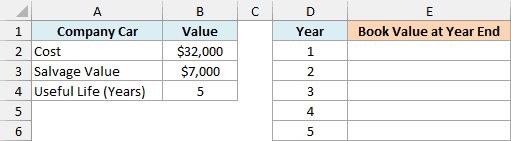
Here is the formula:

=B2-SLN(B2,B3,B4)*D2:D6

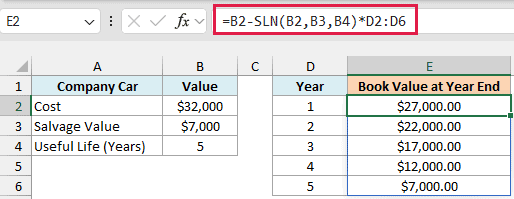
SLN(B2,B3,B4) returns the yearly depreciation of $5,000. Multiplying it by the year number in D2:D6 gives the total depreciation up to the end of that year, and subtracting that from the cost in B2 gives the book value.

So the car is worth $27,000 after year 1, $22,000 after year 2, and so on. In the last year, the book value lands exactly on the $7,000 salvage value, which is a quick way to check that the schedule is right.

The year numbers in column D need to match the useful life in B4. If you change the life to 6 years, add a sixth year in D7 and change D2:D6 in the formula to D2:D7.

If you are using Excel 2019 or earlier, enter the below formula in cell E2 and then copy it down the range:

=$B$2-SLN($B$2,$B$3,$B$4)*D2

Example 5: Depreciation for Assets Bought Partway Through the Year

SLN assumes the asset is in use for the full period. But when you buy something in, say, October, it only gets a few months of depreciation in its first year.

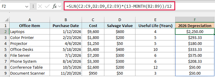
Below is a list of office items bought on different dates in 2026, and I want to get each item’s depreciation for 2026 in column F.

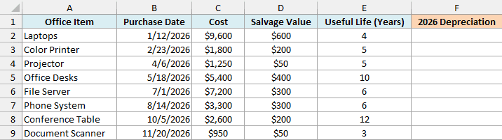
Here is the formula:

=SLN(C2:C9,D2:D9,E2:E9)*(13-MONTH(B2:B9))/12

How this formula works:

• SLN(C2:C9,D2:D9,E2:E9) returns the full yearly depreciation for each item.
• 13-MONTH(B2:B9) counts the months each item was in use in 2026, including the month it was bought. The MONTH function returns the month number of each purchase date, so an item bought in October (month 10) gets 13 – 10 = 3 months.
• /12 turns those months into a fraction of the year, and the yearly depreciation is multiplied by that fraction.

For example, the document scanner bought in November has a yearly depreciation of $300, but it only gets 2 months in 2026, so its 2026 depreciation is $50.00.

Important: This formula counts the purchase month as a full month and assumes your year runs from January to December. Companies handle partial months differently, so check your own rule before using it.

This only applies to the year the asset was bought. From the second year on, the item gets the full yearly amount from SLN.

If you are using Excel 2019 or earlier, enter the below formula in cell F2 and then copy it down the range:

=SLN(C2,D2,E2)*(13-MONTH(B2))/12

Example 6: Total Yearly Depreciation by Department

Let’s step it up with something a bit more advanced. Instead of getting depreciation for each item, this example adds it up for a group of items.

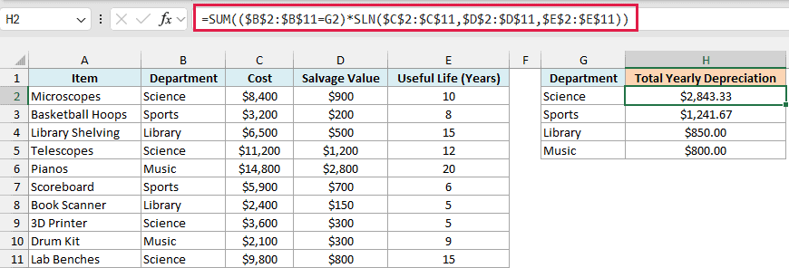
Below is a list of school equipment with the department each item belongs to, and I want to get the total yearly depreciation for each department in column H.

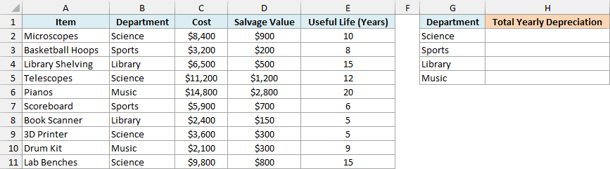
Here is the formula:

=SUM(($B$2:$B$11=G2)*SLN($C$2:$C$11,$D$2:$D$11,$E$2:$E$11))

How this formula works:

• SLN($C$2:$C$11,$D$2:$D$11,$E$2:$E$11) returns the yearly depreciation for all ten items as an array, without needing a helper column.
• ($B$2:$B$11=G2) checks which items belong to the department in G2. It returns TRUE for a match and FALSE for everything else.
• Multiplying the two turns TRUE into 1 and FALSE into 0, so only the depreciation of the matching items is kept.
• SUM then adds up what’s left.

For Science, that’s the microscopes, telescopes, 3D printer, and lab benches, which together lose $2,843.33 a year.

The ranges are locked with dollar signs (absolute references) so you can copy the formula down to get the total for the other departments.

In Excel 2019 or earlier, this SUM formula only works if you enter it with Ctrl + Shift + Enter. The SUMPRODUCT function handles the same array math with a normal Enter.

So in that case, enter the below formula in cell H2 and then copy it down the range:

=SUMPRODUCT(($B$2:$B$11=G2)*SLN($C$2:$C$11,$D$2:$D$11,$E$2:$E$11))

So these are six practical ways to use the SLN function in Excel. It handles one asset or a whole list, gives you yearly or monthly figures, and works well inside other formulas when you need book values or totals.

If you want an asset to lose more value in its early years, the DB and DDB functions use declining-balance methods instead.

I hope you found this Excel tutorial useful.

List of All Excel Functions

Other Excel Articles You May Also Like:

• PMT Function in Excel
• FV Function in Excel
• DDB function
• DB function
• VDB function
• AMORDEGRC function
• AMORLINC Function in Excel
• SYD Function in Excel