

The AMORLINC function in Excel calculates an asset’s depreciation for a chosen accounting period, including a partial first year when you buy it partway through the year.
For example, a scanner bought in April shouldn’t automatically get a full year’s depreciation in December. AMORLINC uses the purchase date and first period’s end date to calculate that first amount, then applies the annual rate in later periods.
Microsoft provides this function for the French accounting system. In this tutorial, I’ll show you how its calculation works, from one asset to a complete schedule and a list of equipment.
Follow along with the example file
AMORLINC Function Examples.xlsx
AMORLINC Function Syntax
Here is the syntax of the AMORLINC function:
=AMORLINC(cost, date_purchased, first_period, salvage, period, rate, [basis])
- cost: The original cost of the asset.
- date_purchased: The date you bought the asset, entered as a real Excel date.
- first_period: The date the first accounting period ends. This is a date, not a period number.
- salvage: The value you expect the asset to retain at the end of its useful life.
- period: The period you want to calculate. Use 0 for the initial purchase-to-period-end interval, 1 for the following annual period, and so on.
- rate: The annual depreciation rate. Enter 20% or 0.2 for a 20% rate, not 20.
- basis (optional): The day-count method used to calculate the partial year. If you leave it out, Excel uses 0.
The first six arguments are required. The square brackets around basis mean that you can omit this argument; you don’t type the brackets in your formula.
These are the supported basis values:
| Basis | Day-count method |
|---|---|
| 0 or omitted | US (NASD) 30/360 |
| 1 | Actual/actual |
| 3 | Actual/365 |
| 4 | European 30/360 |
The two 30/360 methods treat months as 30 days and a year as 360 days, with different month-end rules. The actual methods use calendar days; the choice can change the first-period amount, as Example 3 shows.
AMORLINC is available in desktop Excel, including Microsoft 365, Excel 2024, 2021, 2019, 2016, and Mac. The spilling formulas below require a version with dynamic arrays, such as Microsoft 365, Excel 2024, or Excel 2021.
When to Use the AMORLINC Function
Use this function when you need to:
- Calculate the first partial year’s depreciation under this date-and-rate method.
- Build an annual depreciation schedule that stops at an asset’s salvage value.
- Apply the same accounting dates to several assets with different costs and rates.
Let’s start with one asset, then extend the calculation to several periods.
Example 1: Calculate the First Partial Year
Let’s work through the arguments with a single result.
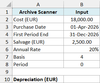
Below are the purchase details for an archive scanner, and I want to calculate its first-period depreciation in cell B10.
Enter the following formula in cell B10:
=AMORLINC(B2,B3,B4,B5,B8,B6,B7)
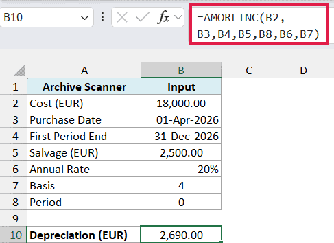
The formula returns 2,690.00, which is the scanner’s depreciation in euros for the first partial year.
Here, B2 supplies the €18,000 cost, B3 the 1-Apr-2026 purchase date, and B4 the 31-Dec-2026 first period end. B5 supplies the €2,500 salvage value, while B8 selects period 0.
The last two arguments use the 20% rate in B6 and European 30/360 basis in B7. Notice that the period, rate, and basis aren’t in worksheet row order, so check their order when building the formula.
A full annual charge would be €18,000 × 20%, or €3,600. For this first interval, basis 4 gives a year fraction of 269/360, so the charge is €3,600 × 269/360 = €2,690.
The salvage value doesn’t get subtracted from the cost before applying the rate. Instead, it limits how much depreciation can be charged over the asset’s life, which we’ll see in the next example.
If either date is stored as unrecognized text, the formula can return #VALUE!. Use real Excel dates in B3 and B4; the DATE function is useful when you need to build a date from separate year, month, and day values.
A first period end before the purchase date gives #NUM!. Check the dates themselves, not just their displayed format, before changing the formula.
Example 2: Build an AMORLINC Depreciation Schedule
Now let’s see what happens after that first partial year.
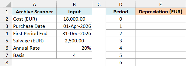
Below are the same scanner details and periods 0 through 6, and I want to calculate each period’s depreciation in column E.
Enter the following formula in cell E2:
=AMORLINC(B2,B3,B4,B5,D2:D8+0,B6,B7)
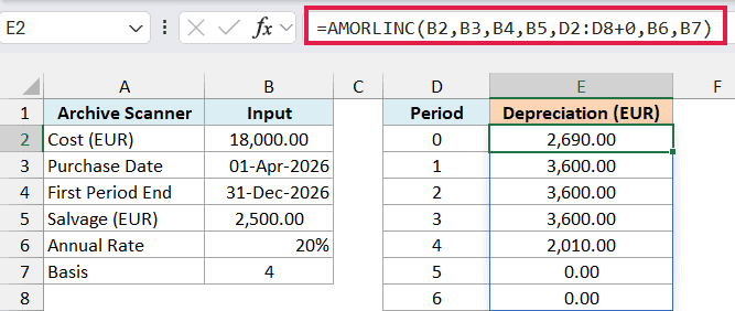
The formula spills seven results into E2:E8. You enter it once, and Excel calculates an amount for each period listed in D2:D8.
There is one extra step when supplying a range: passing D2:D8 directly as the period argument returns #VALUE!. Adding +0 turns those cell references into an array of numeric values that the function can use, without changing the numbers.
Important: Keep the +0 when passing a numeric range to AMORLINC. Also leave the cells below the formula empty so Excel has room for the spilled results.
Period 0 returns €2,690, the partial-year amount from Example 1. Periods 1, 2, and 3 each return €3,600, the full annual charge based on the original cost and rate.
Period 4 returns only €2,010. By then, €13,490 has already been depreciated, and only €2,010 remains before the scanner reaches its €2,500 salvage value.
Periods 5 and 6 return 0 because that limit has been reached. Each result is the depreciation for that period, not the accumulated depreciation or the asset’s remaining value.
Use whole, nonnegative period numbers in this schedule. A negative period returns #NUM!, and Excel truncates a fractional period, so 1.9 calculates period 1 rather than a partial period.
The annual rate must be greater than zero; a zero rate also returns #NUM!. This is different from the valid zero results at the end of the schedule.
If you’re using Excel 2019 or 2016, enter this scalar formula in E2 and copy it down to E8:
=AMORLINC($B$2,$B$3,$B$4,$B$5,D2,$B$6,$B$7)
The dollar signs keep the asset inputs fixed while D2 changes to the next period as you copy the formula down.
Follow along with the example file
AMORLINC Function Examples.xlsx
Example 3: Compare the Day-Count Basis Options
The same purchase dates can produce slightly different first-period amounts.
Below are the scanner details with the four supported basis codes, and I want to compare their period-0 depreciation in column E.
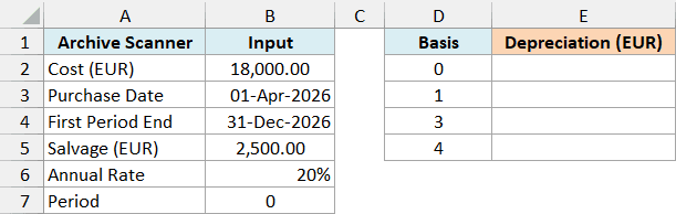
Enter the following formula in cell E2:
=AMORLINC(B2,B3,B4,B5,B7,B6,D2:D5+0)
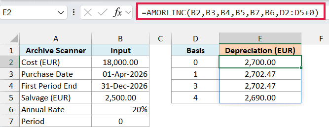
Here, B7 fixes the period at 0, and the last argument supplies the basis codes from D2:D5. The +0 performs the same range-to-array conversion used in the previous example.
Basis 0 returns €2,700.00, while basis 4 returns €2,690.00. Their different month-end conventions produce different year fractions for this interval, even though both use a 360-day year.
Bases 1 and 3 both return €2,702.47 here. The interval contains 274 actual days, and both methods use 365 as the year length in this non-leap-year example.
That matching result doesn’t make the two methods interchangeable. Basis 1 follows the actual year length, while basis 3 uses 365, so a leap-year interval can change the comparison.
Important: AMORLINC does not support basis 2. Entering 2 returns #NUM!, so choose 0, 1, 3, or 4 to match the day-count method your calculation requires.
If you’re using Excel 2019 or 2016, enter this formula in E2 and copy it down to E5:
=AMORLINC($B$2,$B$3,$B$4,$B$5,$B$7,$B$6,D2)
Example 4: Calculate Depreciation for Several Assets
So far, we’ve changed the period or basis for one asset. Now let’s calculate the same period for several assets.
Below is a list of studio equipment bought on the same date, and I want to calculate each item’s first-period depreciation in column E.
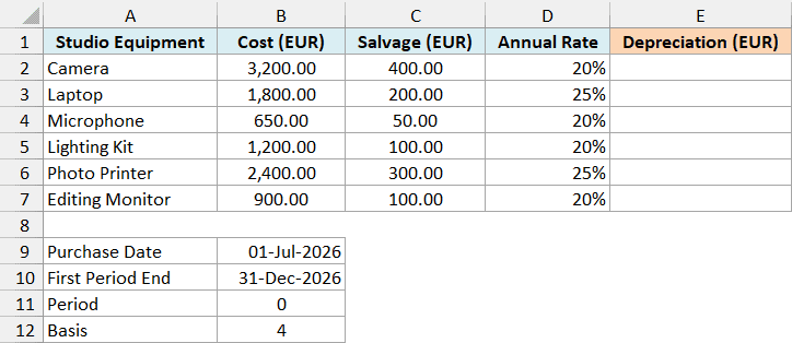
Enter the following formula in cell E2:
=AMORLINC(B2:B7+0,B9,B10,C2:C7+0,B11,D2:D7+0,B12)
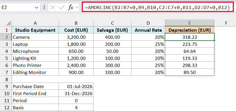
The formula returns one amount per item. For example, the camera gets €318.22, the laptop gets €223.75, and the editing monitor gets €89.50.
The three ranges supply each item’s cost, salvage value, and annual rate. Each range has +0 so AMORLINC receives numeric value arrays, and Excel matches the values by row.
The remaining arguments come from the shared inputs below the equipment list: the 1-Jul-2026 purchase date, 31-Dec-2026 period end, period 0, and basis 4.
For the camera, the full annual charge is €3,200 × 20% = €640. The first interval is 179/360 of a year under basis 4, giving €318.22 when displayed to two decimal places.
Keep the cost, salvage, and rate ranges the same size and aligned with the same assets. A number from the wrong row can still produce a valid-looking result for the wrong item.
If you’re using Excel 2019 or 2016, enter this formula in E2 and copy it down to E7:
=AMORLINC(B2,$B$9,$B$10,C2,$B$11,D2,$B$12)
Here, the shared dates, period, and basis stay fixed, while the cost, salvage value, and rate change for each equipment row.
AMORLINC uses an annual rate and dates. If your calculation instead divides the depreciable cost evenly over a specified useful life, the SLN function uses that different set of inputs.
In this tutorial, I showed you how to calculate a partial first year, build a depreciation schedule, compare basis options, and handle several assets with one formula.
I hope you found this article helpful.
Other Excel Articles You May Also Like:
