
If you have ever wanted one formula to return a whole list of results instead of just a single value, dynamic arrays are exactly what you are looking for.
With dynamic arrays, a single formula can return many values that “spill” into the cells around it automatically. No dragging the formula down, no copy-paste.
In this article, I’ll walk you through what dynamic arrays are, how the spill range works, the new functions that come with them, and a few things that trip people up.
One quick note before we start. Dynamic arrays work in Microsoft 365, Excel 2024, Excel 2021, and Excel for the web, but NOT in Excel 2019, 2016, or earlier, so on an older version these formulas will not work for you.
What Are Dynamic Arrays in Excel
Let’s start with the core idea using a small example.
Say you have a list of cities in cells B2:B11 and you want a separate list of just the unique ones. In the old days, you would copy the column, then run Remove Duplicates, or build a clunky formula and fill it down.
With a dynamic array, you type one formula in a single cell and Excel returns every unique city at once, filling the cells below on its own.
That behavior of one formula returning multiple values and placing them in the neighboring cells is called spilling.
Below is the dataset I’ll use throughout this article. It has a salesperson, a city, a product, and the units sold.
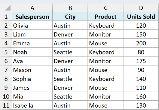
Here is a formula that returns the unique cities:
=UNIQUE(B2:B11)
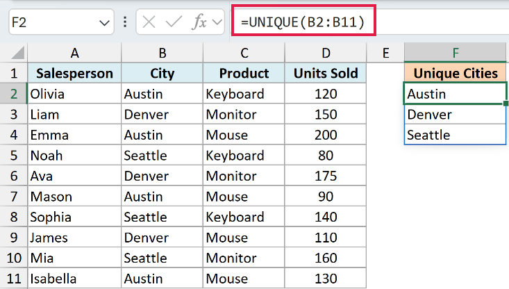
I typed this into a single cell, and Excel returned three cities. Austin, Denver, and Seattle.
They spilled down into the cells below the formula cell automatically.
You only edit the formula in the top cell. The cells below just show the values.
Select any one of them and the formula bar shows a lighter, “ghosted” version of the formula that you cannot edit.
If your source data changes, say you replace one of the cities with a new name, the spilled result updates on its own.
That is the “dynamic” part. The output resizes to match the data.
One thing to note. A fixed range like B2:B11 will not pick up new rows you add below it.
If you want that, convert the data to an Excel Table and use the table column in the formula instead.
Also, spilling is not limited to the new functions. Plain references and arithmetic spill too, because spilling is part of Excel’s calculation engine.
Say every unit in our data sells for $25 and you want the revenue for each row. Instead of writing one formula and dragging it down, you can do it in one go:
=D2:D11*25
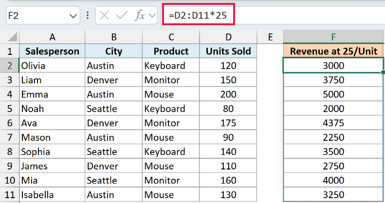
One formula, and Excel multiplies every value in D2:D11 by 25 and spills all ten results down the column.
The Spill Range and the Spilled Range Operator
When a formula spills, the full block of returned values is called the spill range.
Click any cell inside that block and Excel draws a blue border around the whole range. That border is your visual cue that the cells belong to one spilled formula.
The handy part is that you can refer to the entire spill range with one reference. You take the top-left cell of the spill (the anchor cell) and add a hash symbol after it.
So if a formula spills starting in cell A1, then A1# refers to the whole spilled range, however big it grows.
Let’s see this in action. Suppose I put this formula in cell A2:
=SEQUENCE(5)
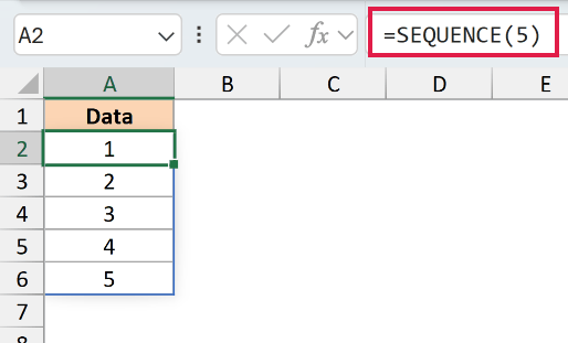
This spills the numbers 1, 2, 3, 4, and 5 down from A2.
Now I can add up that whole spilled range with this:
=SUM(A2#)
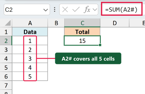
This returns 15, which is the sum of 1 through 5.
The big advantage of A2# is that it always covers the full spill, even when it grows or shrinks. If the spill later returns 8 values instead of 5, A2# picks up all 8 with no edits from you.
Extracting One Column from a Multi-Column Spill
There is one thing about the # reference that trips people up. It always returns the ENTIRE spill, every row and every column of it.
Suppose I use FILTER to pull out all the Austin rows, with the result spilling from cell F2:
=FILTER(A2:D11,B2:B11="Austin")
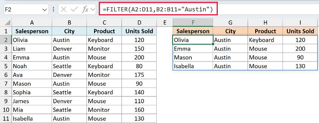
Now say I want to count how many records came back. The obvious formula would be COUNTA:
=COUNTA(F2#)
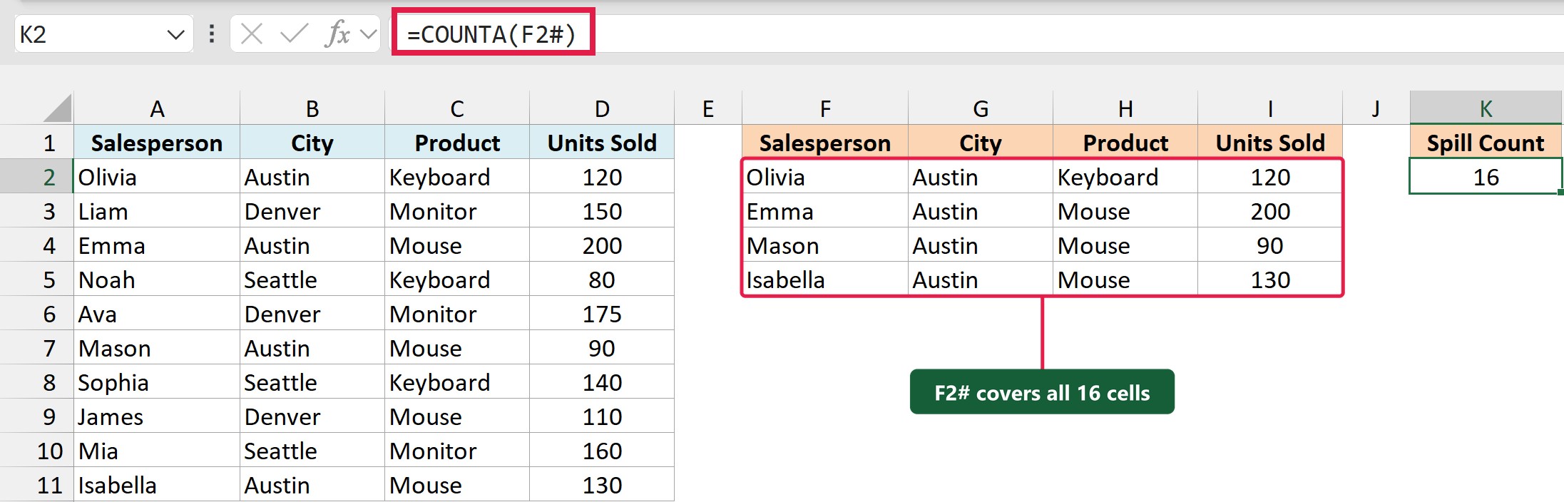
This returns 16, not 4. F2# is the whole block of 4 rows and 4 columns, so COUNTA counts every filled cell in it.
The fix is the INDEX function. If you leave its row argument empty, it returns one full column of the spill:
=INDEX(F2#,,1)
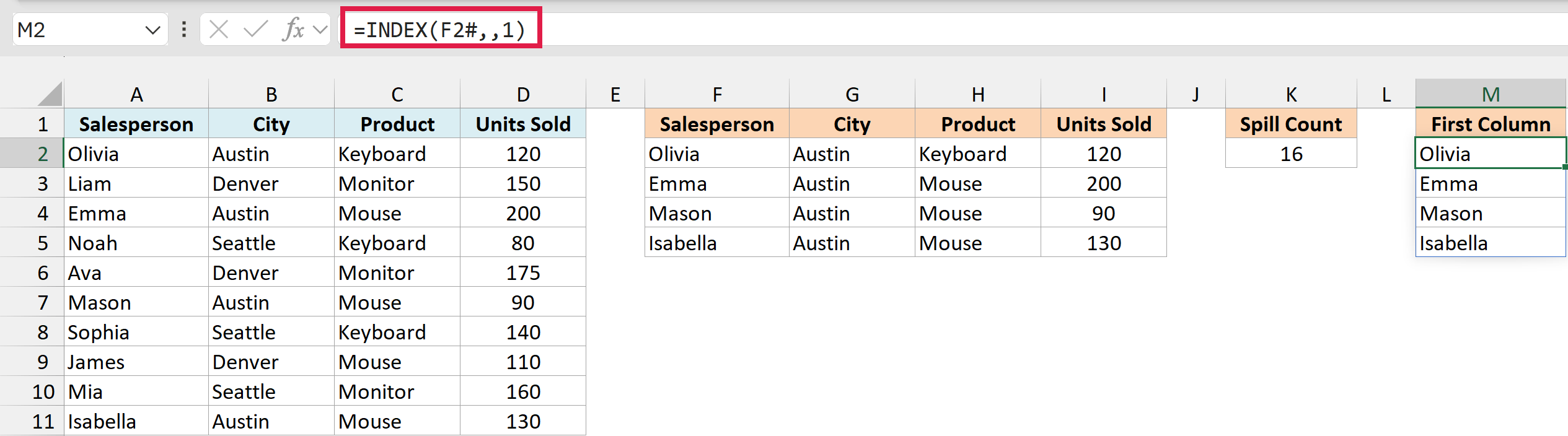
This spills just the first column of the block, which is the four salesperson names.
Wrap that in COUNTA and you get the count you actually wanted:
=COUNTA(INDEX(F2#,,1))
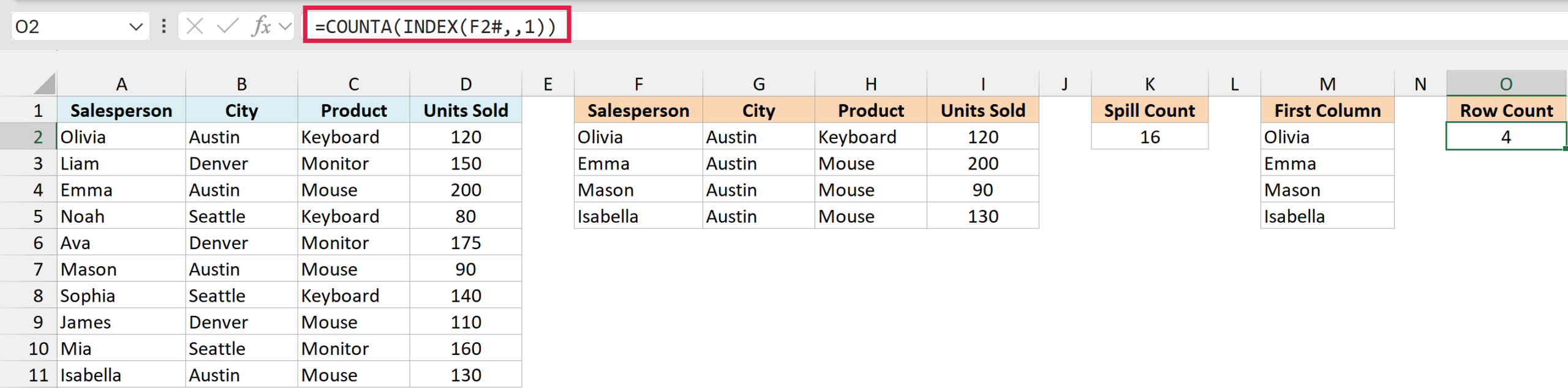
This returns 4, the real number of records.
The #SPILL! Error and How to Fix It
A dynamic array formula needs empty cells to spill into. If something is blocking the area where the results want to land, Excel cannot place them and shows a #SPILL! error instead.
The most common cause is data sitting in the way. If your =UNIQUE(B2:B11) formula needs three cells going down, but one of those cells already has a value typed in it, the spill is blocked.
A merged cell in the spill area causes the same problem. Dynamic arrays cannot spill into merged cells at all.
The fix is simple. Click the formula cell, and Excel shows a dashed border around where the result wants to go.
Find the cell that is in the way inside that border, then clear or move whatever is blocking it.
Once the path is clear, the formula spills as expected and the error goes away.
Pro Tip: Click the small warning icon next to the #SPILL! cell. Excel shows the exact reason (such as “Spill range isn’t blank”) and a Select Obstructing Cells option that jumps straight to the blocker, handy when it’s something invisible like a stray space.
A blocked or merged cell causes most #SPILL! errors, but Excel has a few other reasons too. The warning icon tells you which one you’ve hit:
- “Table formula” means the formula is inside an Excel Table, and Tables don’t support spilled formulas. Move the formula to a normal cell outside the Table, or convert the Table to a range.
- “Extends beyond the worksheet’s edge” means the result needs more rows than the sheet has. A whole-column reference like A:A returns a value for every row of the sheet, so
=A:A*2entered in row 2 runs out of rows. Point the formula at just the cells with data, like A2:A100. - “Indeterminate size” means the size of the result keeps changing while Excel calculates. This happens when a random function decides how many values come back, as in
=SEQUENCE(RANDBETWEEN(1,1000)). - “Out of memory” means the array is too big for Excel to handle. Point the formula at a smaller range.
The New Dynamic Array Functions
A set of functions was built specifically to take advantage of spilling. Here is a quick rundown of each, with a tiny example so you can see what it does.
UNIQUE returns a list of the unique values from a range.
=UNIQUE(B2:B11)
This pulls the distinct cities from our data and spills them: Austin, Denver, Seattle.
SORT sorts a range and spills the sorted result.
=SORT(B2:B11)
This returns the city list in alphabetical order.
SORTBY sorts one range based on the values in another range.
=SORTBY(A2:A11,D2:D11,-1)
This lists the salespeople sorted by their units sold, from highest to lowest. The -1 means descending.
SORT and SORTBY are also how you sort a spilled result. The regular Sort button refuses to touch a spill range and shows a “You can’t change part of an array” message, so build the sorting into the formula instead.
FILTER returns only the rows that meet a condition.
=FILTER(A2:D11,B2:B11="Austin")
This returns every row where the city is Austin.
SEQUENCE generates a list of sequential numbers.
=SEQUENCE(3,3)
This spills a 3 by 3 grid containing the numbers 1 through 9.
RANDARRAY returns an array of random numbers.
=RANDARRAY(5,1,1,100,TRUE)
This spills 5 random whole numbers between 1 and 100 down a single column.
XLOOKUP and XMATCH, the modern replacements for VLOOKUP and MATCH, also work naturally with spilling. XLOOKUP can spill the whole row or column of data for the record it finds, and you can feed it a spilled range as the lookup values.
The six functions above work in Excel 2021 and later. Microsoft has added more array functions since, and these work in Microsoft 365 and Excel 2024, but not in Excel 2021:
- TAKE and DROP keep or remove a set number of rows or columns from the start or end of an array.
- CHOOSECOLS and CHOOSEROWS pull out specific columns or rows by their position.
- VSTACK and HSTACK stack ranges on top of each other or side by side.
- TOCOL and TOROW flatten a range into a single column or row.
- WRAPROWS and WRAPCOLS turn a single row or column into a grid.
- EXPAND pads an array out to a set number of rows and columns.
- TEXTSPLIT splits text into columns or rows at a delimiter.
And these are only in Microsoft 365:
- GROUPBY and PIVOTBY summarize data with one formula, a bit like a PivotTable that spills.
- TRIMRANGE trims the empty rows and columns off the edges of a range, so a big reference does not drag in thousands of blank cells.
A Couple of Worked Examples
Now let’s put a few of these together on the real dataset so you can see how they behave.
Example 1: List the unique cities
I want a clean list of every city that appears, with no repeats. Here is the formula:
=UNIQUE(B2:B11)
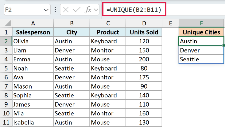
The result spills three values: Austin, Denver, and Seattle. If you would also like them sorted, you can wrap UNIQUE inside SORT, like =SORT(UNIQUE(B2:B11)).
Example 2: Pull all the rows matching a criteria
Now I want every record where the city is Austin, pulled out into its own block. Here is the formula:
=FILTER(A2:D11,B2:B11="Austin")
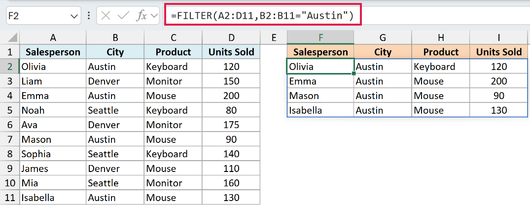
This returns four full rows. Olivia (Keyboard, 120), Emma (Mouse, 200), Mason (Mouse, 90), and Isabella (Mouse, 130).
The result spills across four columns and four rows in one shot, and it updates the moment your source data changes.
If no row matched the condition, FILTER would return a #CALC! error by default. You can avoid that by adding a third argument, like =FILTER(A2:D11,B2:B11="Austin","No match"), which shows your own message instead.
Example 3: Create a dynamic drop-down
Let’s combine what we have covered into something genuinely useful: a drop-down list that maintains itself when your data changes.
First, get the unique cities with UNIQUE, here in cell F2:
=UNIQUE(B2:B11)
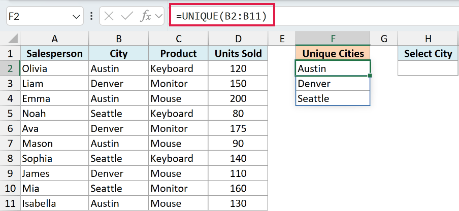
Next, select the cell where you want the drop-down (H2 in my case), go to Data > Data Validation, select List under Allow, and enter this in the Source field:
=$F$2#
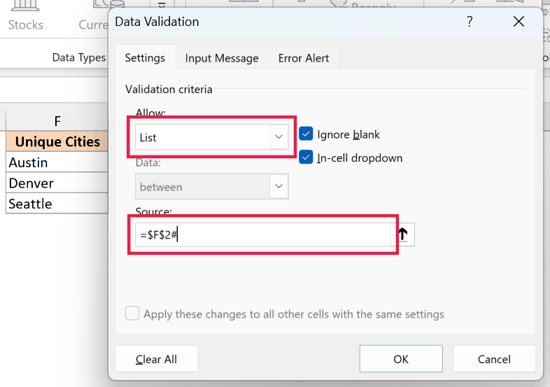
The # is what makes this dynamic. The drop-down follows the spilled list, however it changes.
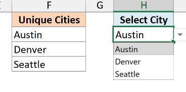
Click OK, and cell H2 now has a drop-down with the three cities.
Finally, enter this FILTER formula in J2 to pull the records for whichever city is selected in H2:
=FILTER($A$2:$D$11,$B$2:$B$11=$H$2)
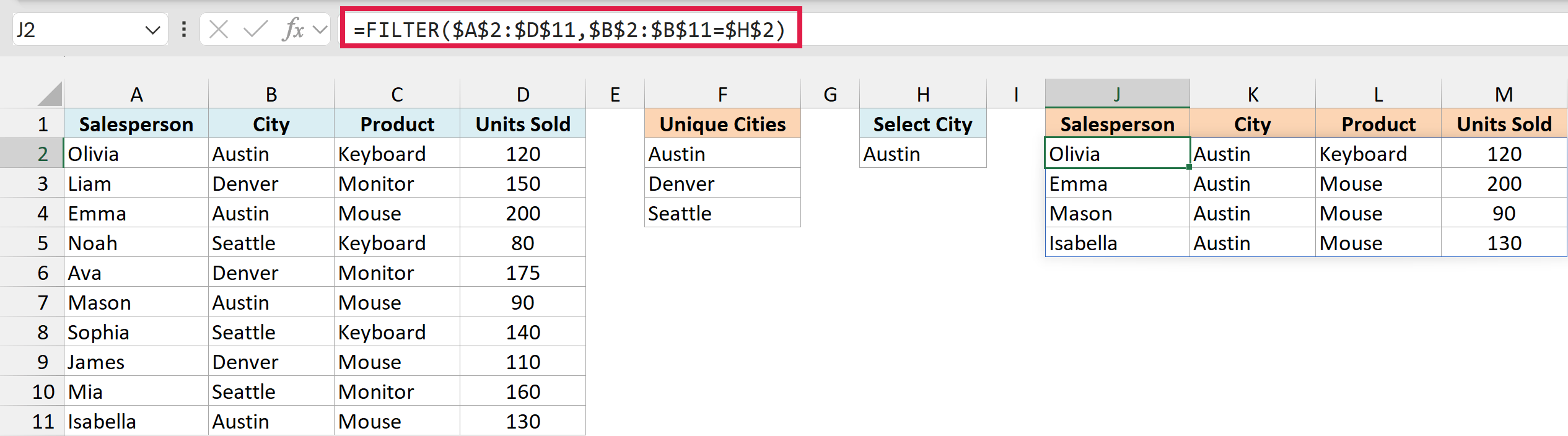
Pick a different city from the drop-down and the results update instantly.
And if a new city ever shows up in B2:B11, UNIQUE picks it up, the drop-down grows on its own, and the filter keeps working.
To also catch rows you add below row 11, convert the data to an Excel Table and use its columns in these formulas.
Implicit Intersection and the @ Operator
Before dynamic arrays existed, Excel quietly handled formulas that returned more than one value through something called implicit intersection.
If a formula could return several values but the cell could only show one, Excel silently picked a single value, the one in the same row (or column) as the formula. This happened in the background, and most people never knew it was there.
Now that Excel can spill, that silent behavior would be confusing. So modern Excel makes it visible using the @ symbol, which is the implicit intersection operator.
When you see @ inside a formula, it means “just give me one value here, do not spill.” For example, =@A2:A11 returns the single value from column A on the formula’s own row, rather than spilling the whole range.
That only works when the formula sits somewhere in rows 2 to 11. Put it in row 20 and you get a #VALUE! error, because A2:A11 has no cell in that row to pick.
Excel sometimes inserts @ automatically when it opens an old workbook, to keep older formulas behaving the way they always did. If you want a formula to spill instead, you can usually delete the @ and let it return the full array.
How This Replaces Old Ctrl+Shift+Enter Array Formulas
If you have used Excel for a while, you may remember pressing Ctrl + Shift + Enter to commit an array formula. Those are often called CSE array formulas.
The catch was that when a formula returned several values, you had to select all the output cells first, and the result was locked to that fixed size. If your data grew, the formula did not.
Dynamic arrays remove all of that. You just press Enter on a single cell and the result spills to whatever size it needs, growing and shrinking with your data automatically.
So in Microsoft 365 and Excel 2021 or later, you almost never need Ctrl + Shift + Enter anymore. A plain dynamic array formula does the same job with far less fuss.
If you send the file to someone on Excel 2019 or older, though, your formulas show up there as old-style CSE array formulas that don’t resize, and functions their version lacks (like UNIQUE) may not calculate.
In this article, I covered what dynamic arrays are, how the spill range and the # operator work, the new functions like UNIQUE, SORT, and FILTER, and how all of this replaces the old Ctrl + Shift + Enter array formulas.
I hope you found this article helpful.
Other Excel Articles You May Also Like: