

The DB function in Excel calculates the depreciation of an asset for a specific year using the fixed-declining balance method. You give it what the asset cost, what it will be worth at the end, and how long it lasts.
Unlike straight-line depreciation, where every year gets the same amount, DB writes off more in the early years and less later on. That’s a good fit for things like vehicles, computers, and machines that lose most of their value soon after you buy them.
In this tutorial, I’ll show you how the DB function works, how to build a full depreciation schedule with one formula, how to handle an asset bought in the middle of the year, and how DB compares with DDB and SLN.
Follow along with the example file
DB Function Examples.xlsx
DB Function Syntax
Here is the syntax of the DB function:
=DB(cost, salvage, life, period, [month])
- cost – what you paid for the asset.
- salvage – what the asset will be worth at the end of its life (also called the salvage value or residual value).
- life – the number of periods over which the asset is depreciated, usually in years.
- period – the period you want the depreciation for, such as 1 for the first year. It must use the same unit as life, so if life is in years, period is in years too.
- [month] – (optional) the number of months in the first year. If you leave it out, Excel uses 12.
DB works out one fixed rate from the cost, salvage, and life, using 1 – (salvage/cost)^(1/life), rounded to three decimal places.
Every year, that same rate is applied to whatever value is left at the start of the year. So the amount goes down each year, even though the rate stays the same.
When month is less than 12, the first year only gets that share of a full year’s depreciation. Example 3 shows how this works for an asset bought in April.
The DB function works in Excel 365, 2024, 2021, 2019, 2016, and older versions, on both Windows and Mac.
When to Use the DB Function
Use this function when you need to:
- Calculate the depreciation of an asset for a particular year using the declining balance method
- Build a depreciation schedule that shows how much an asset loses each year and what it’s worth at year end
- Handle an asset that was bought partway through the year
- Calculate this year’s depreciation for a whole list of equipment at once
- Compare declining balance depreciation with the double-declining balance and straight-line methods
Let me show you a few practical examples of how to use the DB function.
Example 1: Calculate First-Year Depreciation With DB
Let’s start with a simple example.
Below are the details of an electric delivery scooter that cost $2,400 and will be worth $300 after 4 years, and I want to calculate its depreciation for the first year in cell B7.
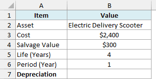
Here is the formula:
=DB(B3,B4,B5,B6)
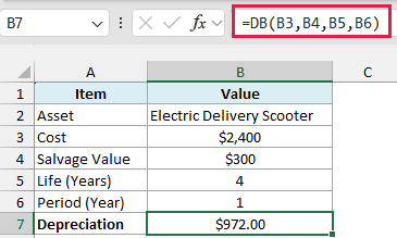
The result is $972.00, which is how much value the scooter loses in its first year.
In the above formula, B3 has the cost, B4 has the salvage value, B5 has the life of 4 years, and B6 has the period (1, for the first year).
Behind the scenes, DB first works out the rate. 1 – (300/2400)^(1/4) is about 0.4054, which Excel rounds to 0.405, and $2,400 multiplied by 0.405 gives you $972.00.
To get the depreciation for a later year, just change the period in B6. Enter 2 there, and you get the second year’s depreciation.
Important: Don’t enter 0 as the salvage value. If you typed 0 in B4, the rate would become 100%, so DB would write off the full $2,400 in the first year and return 0 for every year after that.
Example 2: Create a Depreciation Schedule in Excel With DB
Now let’s see the depreciation for every year of an asset’s life, all from one formula.
Below are the details of a large-format printer for a print shop, along with the years 1 to 5, and I want to get the depreciation for each year in column B and the book value at the end of each year in column C.
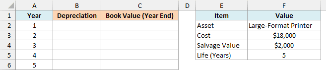
Here is the formula for the depreciation:
=DB(F3,F4,F5,A2:A6)
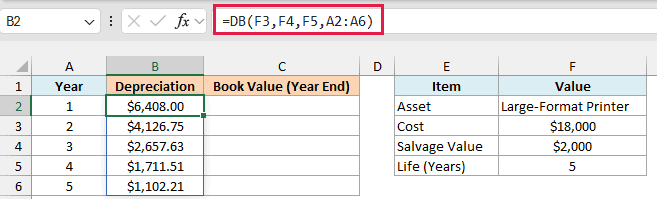
This one formula in B2 spills down to B6 and gives you the depreciation for all five years, starting at $6,408.00 in Year 1 and dropping to $1,102.21 in Year 5.
Instead of a single period, I gave DB the whole list of years in A2:A6. DB calculates the depreciation once for each year and returns all five results together.
If you are using Excel 2019 or earlier, enter the below formula in cell B2 and then copy it down to B6:
=DB($F$3,$F$4,$F$5,A2)
The dollar signs lock the cost, salvage, and life cells, so they don’t shift when you copy the formula down. Only the year reference changes from row to row.
The same fill-down approach works for the spilling formulas in Examples 3 and 6.
Here is the formula for the book value at the end of each year:
=$F$3-SUM($B$2:B2)
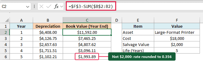
This formula goes in C2 and is copied down to C6. It subtracts all the depreciation up to that year from the cost, so you can see what the printer is worth at the end of each year.
The range $B$2:B2 grows by one row each time you copy the formula down, which makes it a simple running total. That’s why this one stays a per-row formula instead of a spilling one.
Now look at the last book value. After five years, the printer is worth $1,993.89 and not exactly the $2,000 salvage value you entered.
This happens because Excel rounds the rate to three decimal places. The exact rate here is about 0.35561, but DB uses 0.356, and that small difference adds up over five years.
So a DB schedule will usually end a little above or below the salvage value. If you need it to land exactly on the salvage value, adjust the last year’s amount by hand.
Example 3: Depreciation When the Asset Is Bought Mid-Year
In real life, assets don’t always get bought on January 1. This is where the month argument comes in.
Below are the details of a sound system for an event venue that was bought on April 1, 2026, with the number of months it was used in the first year in E7, and I want to get the depreciation for each period in column B.
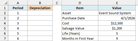
Here is the formula:
=DB(E4,E5,E6,A2:A7,E7)
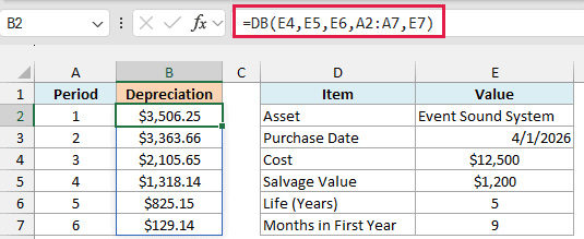
This gives you six results, from $3,506.25 for the first period down to $129.14 for the sixth.
E7 has the number of months the sound system was used in its first year. Since it was bought in April, that’s April to December, so I typed 9 there.
DB doesn’t read the purchase date in E3, so you need to count these months yourself.
With 9 months, the first period only gets 9/12 of a full year’s depreciation. That’s $12,500 multiplied by the rounded rate of 0.374, and then by 9/12, which gives $3,506.25.
The life is still 5 years, which is 60 months. Period 1 uses 9 of them and periods 2 to 5 use 48 more, which leaves 3 months for a sixth period.
That’s why the depreciation in period 6 is so small.
Important: The extra period only works when month is less than 12. If you leave the month argument out, asking for period 6 on a 5-year life returns a #NUM! error.
DB returns the same #NUM! error for other inputs it can’t use. That includes a life or period of 0 or less, a period beyond that extra one, a month below 1 or above 12, and a negative cost or salvage value.
Example 4: Depreciation for a Whole Equipment List in One Formula
Let’s step it up with a more practical use case, where every asset has its own numbers.
Below is the equipment list of a landscaping business, with the cost, salvage value, life, and the year each item is in, and I want to calculate this year’s depreciation for every item in column F.
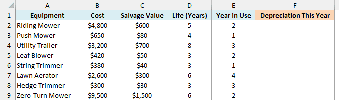
Here is the formula:
=DB(B2:B9,C2:C9,D2:D9,E2:E9)
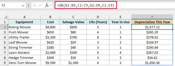
This single formula in F2 spills down to F9 and gives the depreciation for all eight items. For example, the riding mower in its second year gives $1,077.12, and the zero-turn mower gives $1,850.36.
Here, every argument is a range instead of a single cell. DB goes row by row and uses that row’s cost, salvage, life, and year, so each item gets its own rate.
Because the formula covers all eight rows of the list, you only need to update the Year in Use column at the start of each year. The depreciation for every item updates on its own.
If you are using Excel 2019 or earlier, enter the below formula in cell F2 and then copy it down to F9:
=DB(B2,C2,D2,E2)
If any of these cells has text in it, such as “5 years” typed in the Life column, that row returns a #VALUE! error. Keep these as plain numbers.
Example 5: Find the Book Value After a Number of Years
Sometimes you don’t need the full schedule. You just want to know what an asset is worth today.
Below are the details of a camera kit that has been used for 3 years, and I want to get its current book value in cell B7.
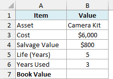
Here is the formula:
=B3-SUM(DB(B3,B4,B5,SEQUENCE(B6)))
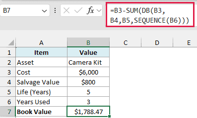
The result is $1,788.47, which is what the camera kit is worth on the books after 3 years.
How this formula works:
- SEQUENCE(B6) creates the list of years 1, 2, and 3, since B6 has 3 years used.
- DB(B3,B4,B5,SEQUENCE(B6)) calculates the depreciation for each of those three years.
- SUM(…) adds up the three amounts to get the total depreciation so far.
- B3-SUM(…) subtracts that total from the $6,000 cost, which leaves the book value.
When the camera kit finishes another year, change B6 to 4 and the book value updates.
The SEQUENCE function needs Excel 365, Excel 2024, or Excel 2021. In older versions, build the year-by-year schedule from Example 2 and read the book value from it.
Example 6: DB vs DDB vs SLN (Declining Balance vs Straight Line)
Excel has a few depreciation functions, and it helps to see them side by side on the same asset.
Below are the details of a rooftop solar panel system, along with the years 1 to 6, and I want to compare the depreciation from DB in column B, DDB in column C, and SLN in column D.
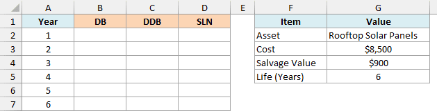
Here is the formula for the DB depreciation:
=DB(G3,G4,G5,A2:A7)
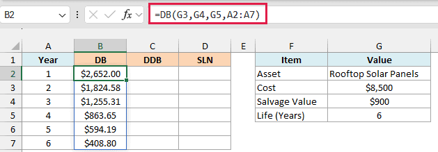
DB starts at $2,652.00 in Year 1 and goes down to $408.80 in Year 6. Its rate comes from the cost, salvage value, and life, and here it works out to 31.2%.
Here is the formula for the DDB depreciation:
=DDB(G3,G4,G5,A2:A7)
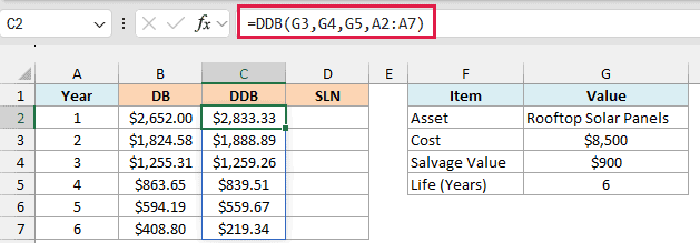
DDB (double-declining balance) starts even higher, at $2,833.33 in Year 1. Its rate doesn’t depend on the salvage value at all, since it’s 2 divided by the life, so 2/6 or about 33.3% here.
DDB also never takes the asset below its salvage value. That’s why its Year 6 amount is only $219.34, which is just enough to bring the value down to exactly $900.
Here is the formula for the SLN depreciation:
=SLN($G$3,$G$4,$G$5)
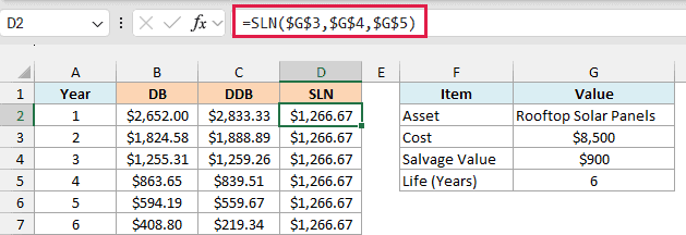
SLN (straight line) gives the same $1,266.67 every year, which is the $7,600 difference between cost and salvage spread evenly over 6 years.
SLN has no period argument, because the answer is the same for every year. So there’s nothing to spill here, and the formula is simply entered in D2 and copied down to D7.
Looking at the three columns together, DB and DDB both front-load the depreciation, while SLN keeps it flat. DB is the one to use when you want a declining balance that’s tied to the salvage value you expect.
So these are some practical examples of using the DB function in Excel to calculate declining balance depreciation. I hope you found this tutorial useful!
Other Excel Articles You May Also Like:
