Excel INDIRECT Function – Overview
The INDIRECT function in Excel can be used when you have the reference of a cell or a range as a text string and you want to get the values from those references.
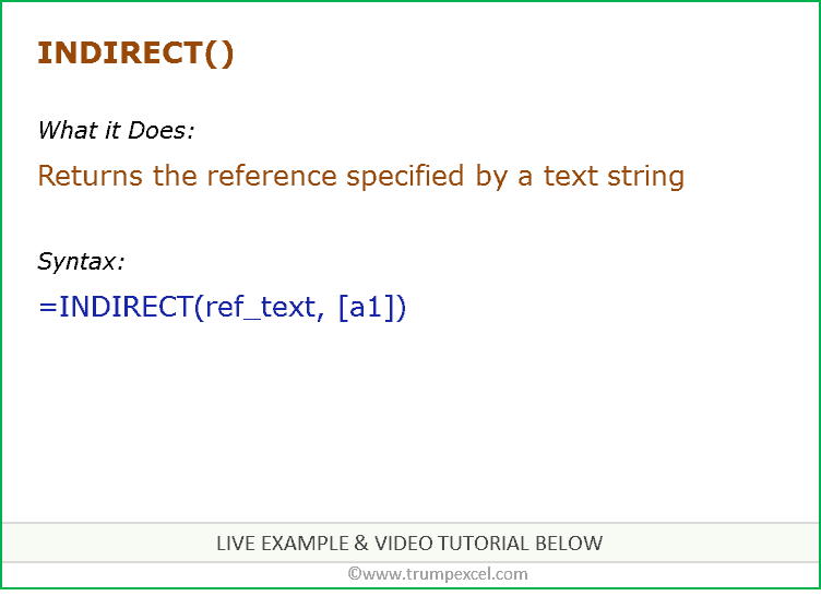
In short – you can use the indirect formula to return the reference specified by the text string.
In this Excel tutorial, I will show you how to use the indirect function in Excel using some practical examples.
But before I get into the examples, let’s first have a look at its syntax.
INDIRECT FUNCTION Syntax
=INDIRECT(ref_text, [a1])
Input Arguments
- ref_text – A text string that contains the reference to a cell or a named range. This must be a valid cell reference, or else the function would return a #REF! error
- [a1] – A logical value that specifies what type of reference to use for ref text. This could either be TRUE (indicating A1 style reference) or FALSE (indicating R1C1-style reference). If omitted, it is TRUE by default.
Additional Notes
- INDIRECT is a volatile function. This means that it recalculates whenever the excel workbook is open or whenever a calculation is triggered in the worksheet. This adds to the processing time and slows down your workbook. While you can use the indirect formula with small datasets with little or no impact on the speed, you may see it making your workbook slower when using it with large datasets
- The Reference Text (ref_text) could be:
- A reference to a cell that in-turn contains a reference in A1-style or R1C1-style reference format.
- A reference to a cell in double-quotes.
- A named range that returns a reference
Examples of How to Use Indirect Function in Excel
Now let’s dive in and have a look at some examples on how to use the INDIRECT function in Excel.
Example 1: Use a Cell reference to Fetch the Value
It takes the cell reference as a text string as input and returns the value in that reference (as shown in the example below):
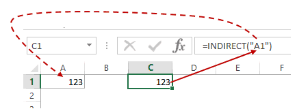
The formula in cell C1 is:
=INDIRECT("A1")
The above formula takes the cell reference A1 as the input argument (within double quotes as a text string) and returns the value in this cell, which is 123.
Now if you’re thinking, why don’t I simply use =A1 instead of using the INDIRECT function, you have a valid question.
Here is why…
When you use =A1 or =$A$1, it gives you the same result. But when you insert a row above the first row, you would notice that the cell references would automatically change to account for the new row.
You can also use the INDIRECT function when you want to lock the cell references in such a way that it does not change when you insert rows/columns in the worksheet.
Example 2: Use Cell Reference in a Cell to Fetch the Value
You can also use this function to fetch the value from a cell whose reference is stored in a cell itself.
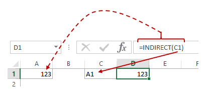
In the above example, cell A1 has the value 123.
Cell C1 has the reference to the cell A1 (as a text string).
Now, when you use the INDIRECT function and use C1 as the argument (which in turn has a cell address as a text string in it), it would convert the value in cell A1 into a valid cell reference.
This, in turn, means that the function would refer to cell A1 and return the value in it.
Note that you don’t need to use double quotes here as the C1 has the cell reference stored in the text string format only.
Also, in case the text string in cell C1 is not a valid cell reference, the Indirect function would return the #REF! error.
Example 3: Creating a Reference Using Value in a Cell
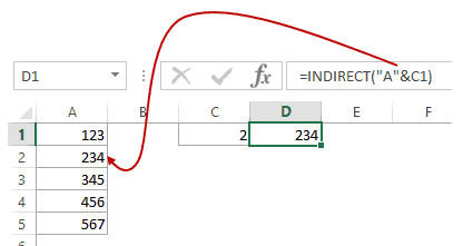
You can also create a cell reference using a combination of the column alphabet and the row number.
For example, if cell C1 contains the number 2, and you use the formula =INDIRECT(“A”&C1) then it would refer to cell A2.
A practical application of this could be when you want to create dynamic reference to cells based on the value in some other cell.
In case the text string you use in the formula gives a reference that Excel doesn’t understand, it will return the ref error (#REF!).
Example 4: Calculate the SUM of a Range of Cells
You can also refer to a range of cells the same way you refer to a single cell using the INDIRECT function in Excel.
For example, =INDIRECT(“A1:A5”) would refer to the range A1:A5.
You can then use the SUM function to find the total or the LARGE/SMALL/MIN/MAX function to do other calculations.

Just like the SUM function, you can also use functions such as LARGE, MAX/MIN, COUNT, etc.
Example 5: Creating Reference to a Sheet Using the INDIRECT Function
The above examples covered how to refer a cell in the same worksheet. You can also use the INDIRECT formula to refer to a cell in some other worksheet or another workbook as well.
Here is something you need to know about referring to other sheets:
- Let’s say you have a worksheet with the name Sheet1, and within the sheet in the cell A1, you have the value 123. If you go to another sheet (let’s say Sheet2) and refer to cell A1 in Sheet1, the formula would be: =Sheet1!A1
But..
- If you have a worksheet that contains two or more than two words (with a space character in between), and you refer to cell A1 in this sheet from another sheet, the formula would be: =’Data Set’!A1
In case, of multiple words, Excel automatically inserts single quotation marks at the beginning and end of the Sheet name.
Now let’s see how to create an INDIRECT function to refer to a cell in another worksheet.
Suppose you have a sheet named Dataset and cell A1 in it has the value 123.
Now to refer to this cell from another worksheet, use the following formula:
=INDIRECT("'Data Set'!A1")
As you can see, the reference to the cell needs to contain the worksheet name as well.
If you have the name of the worksheet in a cell (let’s say A1), then you can use the following formula:
=INDIRECT("'"&A1&"'!A1")

If you have the name of the worksheet in cell A1 and cell address in cell A2, then the formula would be:
=INDIRECT("'"&A1&"'!"&A2)
Similarly, you can also modify the formula to refer to a cell in another workbook.
This could be useful when you trying to create a summary sheet that pulls the data from multiple different sheets.
Also remember, when using this formula to refer to another workbook, that workbook must be open.
Example 6: Referring to a Named Range Using INDIRECT Formula
If you have created a named range in Excel, you can refer to that named range using the INDIRECT function.
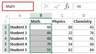
For example, suppose you have the marks for 5 students in three subjects as shown below:

In this example, let’s name the cells:
- B2:B6: Math
- C2:C6: Physics
- D2:D6: Chemistry
To name a range of cells, simply select the cells and go to the name box, enter the name and hit enter.
Now you can refer to these named ranges using the formula:
=INDIRECT("Named Range")
For example, if you want to know the average of the marks in Math, use the formula:
=AVERAGE(INDIRECT("Math"))
If you have the named range name in a cell (F2 in the example below has the name Math), you can use this directly in the formula.
The below example shows how to calculate the average using the named ranges.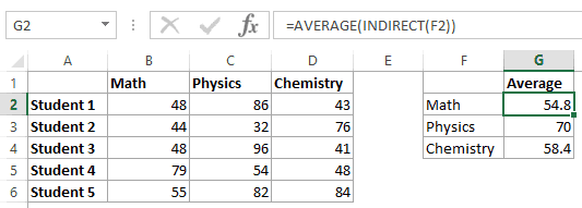
Example 7: Creating a Dependent Drop Down List Using Excel INDIRECT Function
This is one excellent use of this function. You can easily create a dependent drop-down list using it (also called the conditional drop-down list).
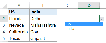
For example, suppose you have a list of countries in a row and the name of cities for each country as shown below:
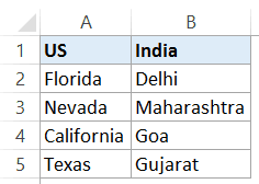
Now to create a dependent drop-down list, you need to create two named ranges, A2:A5 with the name US and B2:B5 with the name India.
Now select cell D2 and create a drop-down list for India and the US. This would be the first drop-down list where the user gets the option to select a country.
Now to create a dependent drop-down list:
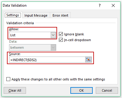
- Select cell E2 (the cell in which you want to get the dependent drop-down list).
- Click the Data tab
- Click on Data validation.
- Select List as the Validation Criteria and use the following formula in the source field: =INDIRECT($D$2)

- Click OK.
Now, when you enter the US in cell D2, the drop-down in cell E2 will show the states in the US.
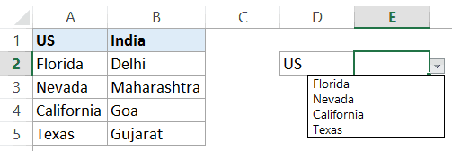
And when you enter India in cell D2, the drop-down in cell E2 will show the states in India.
So these are some examples to use the INDIRECT function in Excel. These examples would work on all the versions of Excel (Office 365, Excel 2019/2016/2013/2013)
I hope you found this tutorial useful.
Related Microsoft Excel Functions:
- Excel VLOOKUP Function.
- Excel HLOOKUP Function.
- Excel INDEX Function.
- Excel MATCH Function.
- Excel OFFSET Function.
You May Also Like the Following Excel Tutorials: