

The ISO.CEILING function rounds a number up to the next whole number, or up to the next multiple of a number you choose, like 5, 10, or 1,000. Up always means toward the larger number, so 4.3 becomes 5 and -4.3 becomes -4.
That makes it useful whenever a partial amount has to count as a full one, like billing for every started mile.
Below, I’ll show you how it works and five practical examples, including one with negative numbers, where the results can surprise you.
Follow along with the example file
ISO.CEILING Function Examples.xlsx
ISO.CEILING Function Syntax
Here is the syntax of the ISO.CEILING function:
=ISO.CEILING(number, [significance])
- number – The value you want to round up. This can be a number, a cell reference, a range, or a calculation.
- significance – (Optional) The multiple you want to round up to, such as 0.1, 10, or 1,000. If you leave it out, Excel uses 1, so the number is rounded up to the next whole number.
ISO.CEILING always rounds toward the larger number. With negative numbers, that means moving toward zero, so -4.3 returns -4, not -5.
The sign of significance doesn’t matter, because Excel only uses its absolute value. So =ISO.CEILING(4.3,-2) returns 6, the same as =ISO.CEILING(4.3,2).
If significance is 0, the function returns 0 instead of an error. If either argument is text that isn’t a number, you get a #VALUE! error.
The ISO.CEILING function works in Excel for Microsoft 365, Excel 2024, 2021, 2019, and 2016, Excel for Mac, and Excel for the web.
When to Use the ISO.CEILING Function
Use this function when you need to:
- Round a number up to the next whole number, like billing every started mile
- Round up to a multiple such as 10, 1,000, or 0.1
- Round up the result of a calculation, like seconds converted to minutes
- Round up a list of numbers that includes both positive and negative values
Let me show you a few practical examples of how to use the ISO.CEILING function in Excel.
Example 1: Round Up to the Next Whole Number
Let’s start with a simple example.
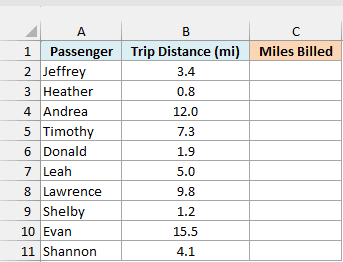
Below is a list of taxi passengers with the distance of each trip, and since the taxi charges for every started mile, I want the billed miles in column C.
Here is the formula:
=ISO.CEILING(B2:B11)
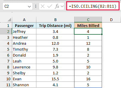
There’s no significance in this formula, so ISO.CEILING rounds each distance up to the next whole number. Jeffrey’s 3.4 miles becomes 4, and Heather’s short 0.8-mile trip still counts as 1.
Andrea’s trip was exactly 12.0 miles, so it stays at 12. A number that’s already whole doesn’t get pushed up.
You only enter this formula in cell C2. In Excel 365, Excel 2024, and Excel 2021, it spills the results down to C11 on its own, and the same goes for every example below.
If you are using Excel 2019 or earlier, enter the below formula in cell C2 and then copy it down the range:
=ISO.CEILING(B2)
The same copy-down approach works for every example below. When the formula points at an input cell, lock that cell with dollar signs, like $F$1, so it doesn’t shift as you copy down.
Example 2: Round Up to a Multiple (Like 1,000)
Now let’s round up to a multiple instead of a whole number.
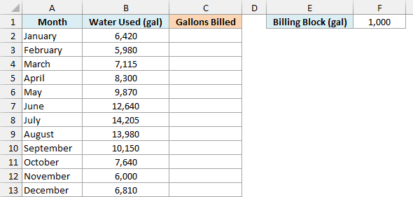
Below is a year of water usage in gallons, and the water company bills in blocks of 1,000 gallons, so I want the billed gallons in column C. The block size is in cell F1.
Here is the formula:
=ISO.CEILING(B2:B13,F1)
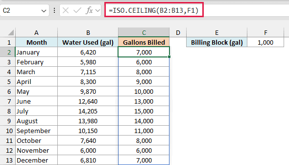
The second argument is the multiple to round up to. F1 holds 1,000, so January’s 6,420 gallons goes up to 7,000, and July’s 14,205 goes up to 15,000.
November’s usage is exactly 6,000, which is already a multiple of 1,000, so it stays at 6,000.
Because the block size sits in a cell, you can change it to 500 or 100 and every result updates. Just don’t leave that cell empty.
Important: A blank cell counts as 0 for significance, so every result in column C would turn into 0 instead of showing an error.
Example 3: Round Up to a Decimal (Like 0.1)
The multiple doesn’t have to be a whole number either. A decimal like 0.1 works the same way.
Below are the lap times in seconds for ten runners, and I want each time rounded up to the next tenth of a second in column C.
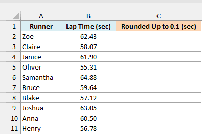
Here is the formula:
=ISO.CEILING(B2:B11,0.1)
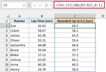
With a significance of 0.1, the possible results are 58.1, 58.2, 58.3, and so on. So Zoe’s 62.43 seconds goes up to 62.5.
Janice’s 61.90 is already on a tenth, so it stays at 61.9. I formatted column B with two decimals and column C with one, so you can see the rounding clearly.
Example 4: Round Up the Result of a Calculation
The number you give ISO.CEILING doesn’t have to be a plain value. It can be a calculation too.
Below is a list of videos with their length in seconds, and I want the length in whole minutes in column C, counting a part of a minute as a full one.
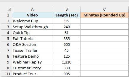
Here is the formula:
=ISO.CEILING(B2:B11/60)
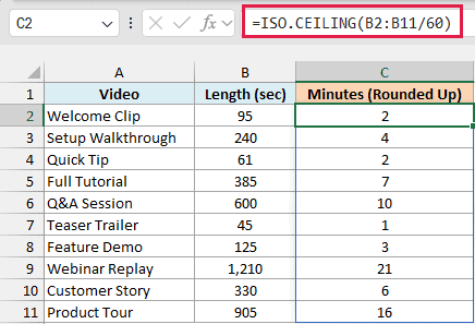
Excel first divides every length by 60 to get minutes, so the Welcome Clip’s 95 seconds becomes 1.58 minutes. ISO.CEILING then rounds that up to 2.
The Q&A Session is exactly 600 seconds, which is 10 minutes with nothing left over, so it stays at 10. And the Quick Tip at 61 seconds goes up to 2, because it runs one second into a second minute.
Example 5: Round Up Negative Numbers
Here is where ISO.CEILING can catch you off guard.
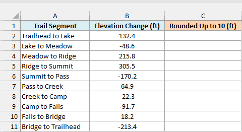
Below is the elevation change for each segment of a hiking trail, with climbs as positive numbers and descents as negative ones, and I want each value rounded up to a multiple of 10 feet in column C.
Here is the formula:
=ISO.CEILING(B2:B11,10)
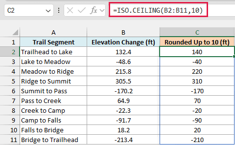
The climbs round up the way you would expect, so 132.4 becomes 140. The descents also round up, which means toward zero, so -48.6 becomes -40 and not -50.
On a number line, up is always to the right. Since -40 is to the right of -48.6, that’s the result you get.
Now let’s check that the sign of significance really is ignored. Enter the below formula in cell D2, which uses -10 instead of 10:
=ISO.CEILING(B2:B11,-10)
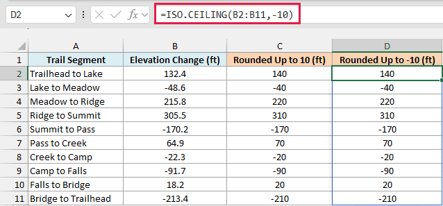
Column D matches column C on every row. A significance of -10 gives the same results as 10.
The older CEILING function can’t do this. It returns a #NUM! error when the number is positive and the significance is negative.
Pro Tip: If you’d rather round negative numbers away from zero (-48.6 to -50), use the CEILING.MATH function and put 1 in its third argument, the mode. For example, =CEILING.MATH(-48.6,10,1) returns -50.
So these are five ways to use the ISO.CEILING function in Excel. It rounds a number up to the next whole number or to any multiple you pick, and with negative numbers, up always means toward zero.
If you’ve used the CEILING.PRECISE function, you already know how this one behaves, because both return the same results.
I hope you found this tutorial useful.
Other Excel Articles You May Also Like:
