

The ISPMT function calculates the interest for a loan payment when you repay the same amount of principal each period. Principal is the amount you borrowed, before interest.
As you pay that principal back, the remaining balance gets smaller, so the interest falls too. Your total payment changes even though the principal portion stays the same.
In this tutorial, I’ll show you how to calculate annual and monthly interest, work from the lender’s perspective, and total the interest for a budget.
Follow along with the example file
ISPMT Function Examples.xlsx
ISPMT Function Syntax
Here is the syntax of the ISPMT function. All four arguments are required:
=ISPMT(rate,per,nper,pv)
- rate is the interest rate for one payment period. Use an annual rate for annual payments or a monthly rate for monthly payments.
- per is the period you want to calculate, starting at 0. The first payment uses 0, the second uses 1, and the last uses
nper-1. - nper is the total number of payment periods for the entire loan.
- pv is the original loan amount. A positive amount represents money the borrower receives and produces negative interest payments; a negative amount represents money lent out and produces positive interest receipts.
Make sure the rate and period count use the same units. For monthly payments with a nominal annual rate, divide that rate by 12 and give nper in months.
ISPMT works in Excel 365, 2024, 2021, 2019, 2016, Mac, and the web. The spilling formulas below need Excel 365, 2024, 2021, or the web; older-version alternatives are included.
When to Use the ISPMT Function
Use this function when you need to:
- Work out interest on a loan with equal principal repayments.
- Calculate a lender’s interest receipts for a particular payment period.
- Budget for interest over several periods of an equal-principal loan.
If your loan has a fixed total payment, including both principal and interest, use the IPMT function to calculate its interest portion. That repayment schedule has different interest amounts because the principal portion changes each period.
Let’s work through the examples.
Example 1: Calculate Annual Interest
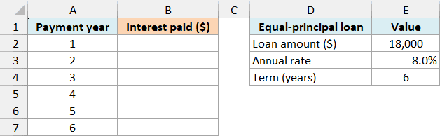
Suppose you borrow $18,000 for equipment at 8% a year and repay $3,000 of principal at the end of each year for six years. Interest is charged on the balance before that year’s principal repayment.
Below is the payment schedule for this equal-principal loan, and I want to calculate the interest paid each year in column B.
On the Annual Interest sheet, enter this formula in cell B2:
=ISPMT(E3,A2:A7-1,E4,E2)
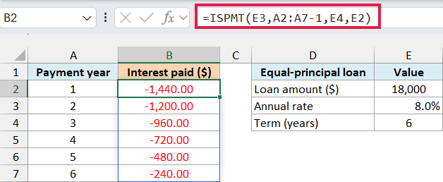
The formula spills six results down column B. The first is -1,440.00, which is 8% of the original $18,000 balance.
After you repay $3,000 of principal, the next year’s opening balance is $15,000. Its interest is $1,200, and the final year’s interest is $240 on the remaining $3,000.
The negative results show money leaving the borrower’s pocket. These amounts contain only interest, so the first total payment would be $3,000 of principal plus $1,440 of interest.
In the formula, A2:A7-1 changes the displayed payment years 1 through 6 into the periods 0 through 5 that ISPMT expects. E3 supplies the rate, E4 supplies the six-year term, and E2 supplies the original loan amount.
Important: Keep the payment numbers between 1 and the loan’s total number of payments when using this formula. ISPMT doesn’t reject periods outside the schedule, so an incorrect number can produce a plausible but wrong result.
For example, passing 6 directly as per on this six-year loan returns zero. The sixth payment actually needs per equal to 5, which is why the formula subtracts 1.
If you see a #SPILL! error, something is blocking the result cells below B2. Move that content out of the way so Excel can display all six results.
If you use Excel 2019 or earlier, enter this formula in B2 and copy it down through B7:
=ISPMT($E$3,A2-1,$E$4,$E$2)
The dollar signs keep the loan inputs fixed while the payment-year reference changes as you copy down.
Example 2: Calculate Monthly Interest
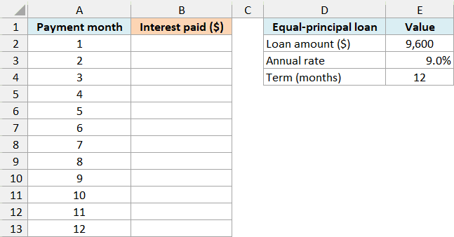
Now suppose an appliance loan is repaid with $800 of principal each month. The original balance is $9,600, the term is 12 months, and the nominal annual rate is 9%.
Below is the schedule for this equal-principal loan, and I want to calculate each month’s interest in column B.
On the Monthly Interest sheet, enter this formula in B2:
=ISPMT(E3/12,A2:A13-1,E4,E2)
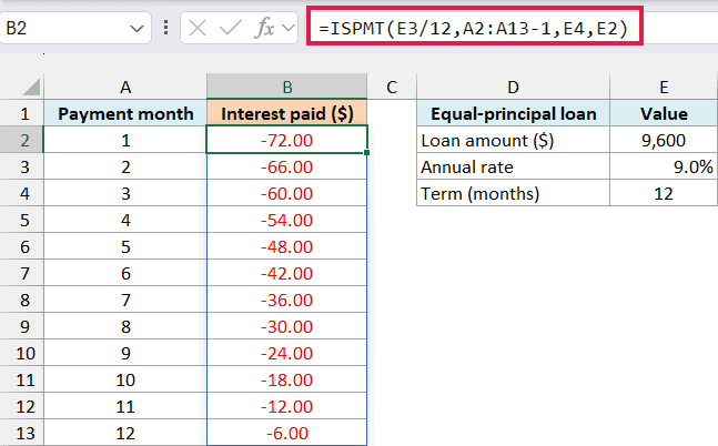
This returns -72.00 for the first month, -66.00 for the second, and progressively smaller amounts down to -6.00 for month 12.
Here, E3/12 converts the nominal annual rate of 9% into a monthly rate of 0.75%. E4 already contains 12 months, so there’s no need to multiply the term by 12 again.
Each $800 principal repayment reduces the next month’s interest by $6. The first total payment is therefore $872, while the last is $806.
Important: Dividing by 12 assumes your annual rate is quoted as a nominal rate with a corresponding monthly rate. If your loan gives an effective annual rate or calculates interest daily, confirm its periodic-rate calculation before using this formula.
Keep the loan inputs numeric. Text such as “nine percent” causes #VALUE!, and a zero term causes #DIV/0! because there’s no valid number of periods over which to repay the principal.
For Excel 2019 or earlier, enter this formula in B2 and copy it down through B13:
=ISPMT($E$3/12,A2-1,$E$4,$E$2)
Example 3: Calculate Interest a Lender Receives
You can also use ISPMT when you’re lending money. The initial amount goes out of your account, while the interest comes back in.
Below are six loans with equal annual principal repayments, and I want the interest received in each loan’s specified payment year in column F.
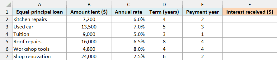
On the Lender Interest sheet, enter this formula in F2:
=ISPMT(C2:C7,E2:E7-1,D2:D7,-B2:B7)
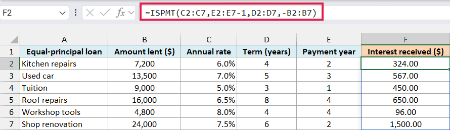
The results spill down column F, with one interest receipt for each loan. The kitchen repairs loan returns $324 for its second payment year.
That loan starts at $7,200 and repays $1,800 of principal each year over four years. After the first repayment, $5,400 remains, so the second year’s interest is 6% of $5,400, or $324.
The minus sign in -B2:B7 treats each amount lent as money paid out. ISPMT then returns positive interest receipts, using each row’s own rate, term, and payment year.
This is a list of separate loans, so the six results are not six consecutive payments on one loan. Keep the four input ranges aligned so each result uses the details from the same row.
For Excel 2019 or earlier, enter this formula in F2 and copy it down through F7:
=ISPMT(C2,E2-1,D2,-B2)
Example 4: Budget for Six Months of Interest
For a budget, you may want interest expenses displayed as positive amounts. Let’s use a $14,400 repair loan with equal monthly principal repayments over 12 months and a nominal annual rate of 10%.
Below are the first six payment months, and I want to calculate their interest expenses in column B and the combined cost in B9.
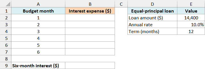
On the Interest Budget sheet, enter this formula in B2:
=-ISPMT(E3/12,A2:A7-1,E4,E2)
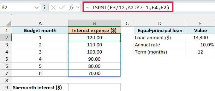
This returns expenses of $120, $110, $100, $90, $80, and $70. The minus sign before ISPMT reverses its negative borrower payments so the budget shows positive costs.
Notice that E4 still contains 12, the full loan term. We’re calculating six months of interest, but the principal is still being repaid over 12 months.
To add those expenses, enter this formula in B9:
=SUM(B2:B7)
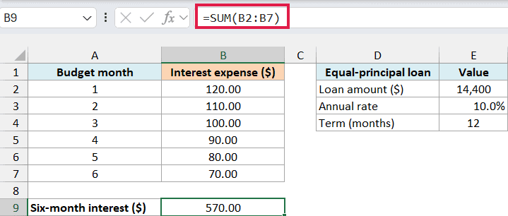
The SUM function returns $570, the interest cost for the first six months. It adds the displayed monthly expenses, so you can check the total against the schedule above it.
This total excludes the principal repayments and any fees. The positive values are a way to present expenses in a budget; they don’t turn those payments into income.
For Excel 2019 or earlier, enter this formula in B2 and copy it down through B7, then use the same SUM formula in B9:
=-ISPMT($E$3/12,A2-1,$E$4,$E$2)
These examples show how to use ISPMT for loans with equal principal repayments. Keep the payment numbering and rate units consistent, and you can use the same approach for your own schedule.
Other Excel Articles You May Also Like:
