

The ISREF function in Excel checks whether an argument is a cell or range reference and returns TRUE or FALSE. It’s useful when a formula builds a reference from text and you want to check whether that reference is valid.
ISREF checks the reference itself, so a blank cell or a cell containing an error can still return TRUE. Giving it a whole range produces one answer, not a separate answer for every cell.
In this tutorial, I’ll show you how these checks work and how to use ISREF to check addresses and worksheet names stored as text.
Follow along with the example file
ISREF Function Examples.xlsx
ISREF Function Syntax
Here is the syntax of the ISREF function:
=ISREF(value)
- value is required. It is the argument you want to test, such as a cell reference, range, defined name, literal value, or the result of another function.
A defined name returns TRUE when it refers to cells. A name that holds a number or text instead is not a reference.
The ISREF function is available in Excel 365, 2024, 2021, 2019, 2016, Mac, and Excel for the web.
When to Use the ISREF Function
Use ISREF when you need to:
- Check whether an argument is a reference rather than a value.
- Check whether an address stored as text can become a valid reference.
- Check a list of worksheet names against the sheets in your workbook.
Let me show you how this works, starting with a direct cell reference.
Example 1: Check a Cell Reference
On the Reference Checks sheet, the sample entries include numbers, text, a blank, and an error, and we want to check their cell references in column C.
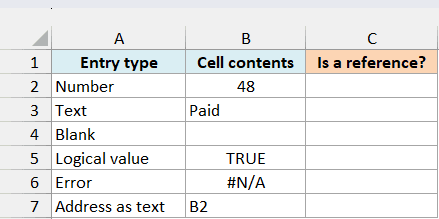
Enter the below formula in cell C2, then copy it down to C7:
=ISREF(B2)
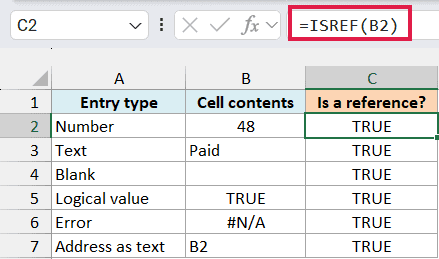
Every row returns TRUE because each formula points to a real cell. B2 contains 48, B3 contains Paid, and B4 is blank, but all three are valid references.
The #N/A error in B6 also returns TRUE in column C. The cell exists, even though its contents are an error.
The text B2 in B7 doesn’t change the test either. The formula in C7 checks the reference to B7, not the address written inside it.
Important: TRUE does not mean the cell contains usable data. ISREF checks the reference; use the ISERROR function when you need to check whether a cell’s contents are an error.
We copy this formula down because each row is a separate reference check. The next example shows what happens if you give ISREF the whole range at once.
Example 2: Check a Whole Range
On the Range Check sheet, we have a small office-supply list and want to check the quantity range, with the answer in E2.
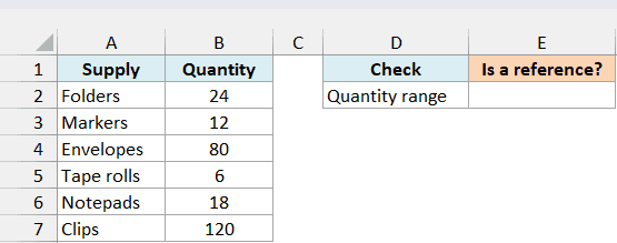
Enter the below formula in cell E2:
=ISREF(B2:B7)
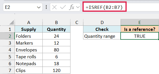
The result is TRUE because B2:B7 is a valid range reference. ISREF treats that entire range as one argument, so it returns one answer in E2.
Important: This formula does not spill six results, even in Excel 365. It also does not check whether the six quantities are numbers or whether any cells are blank.
You can change a quantity or clear one of the cells and the reference will still be valid. If a reference inside a formula becomes #REF! after its cells are deleted, ISREF returns FALSE for that broken reference.
Example 3: Validate Addresses Stored as Text
An address written in a cell is text until a formula converts it to a reference. Passing the quoted text “B2” directly to ISREF returns FALSE, even though B2 is a valid cell address.
The Address Checks sheet contains a list of address strings, and we want to show in column B which ones resolve to valid references.
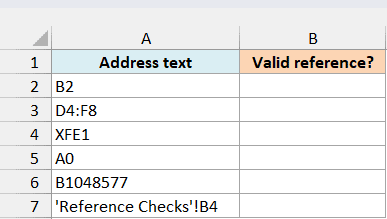
Enter the below formula in B2, then copy it down to B7:
=ISREF(INDIRECT(A2))
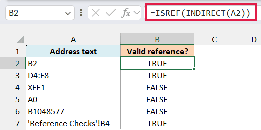
The INDIRECT function reads the text in A2 and tries to turn it into a reference. ISREF then checks that reference, so B2 and D4:F8 both return TRUE.
The three invalid addresses return FALSE for different reasons:
- XFE1 is beyond Excel’s last column, XFD.
- A0 uses row zero, but Excel’s rows start at 1.
- B1048577 is beyond Excel’s last row, 1,048,576.
The last address points to B4 on the Reference Checks sheet. That cell is blank, but the address still returns TRUE because the cell reference is valid.
When INDIRECT cannot resolve an address, it returns #REF!, and ISREF returns FALSE. You don’t need an IFERROR wrapper just to turn that invalid reference into FALSE.
We check one address per row here. Passing the list of address strings to these functions at once does not produce the same set of individual reference checks.
INDIRECT is volatile, which means it recalculates whenever Excel recalculates. It’s useful here because the addresses are stored as text, but avoid copying this formula into thousands of unused rows.
Example 4: Check Whether Worksheets Exist
You can use the same idea for a worksheet checklist by building a reference to A1 on each sheet.
The Owner’s List sheet contains the worksheet names to check, and we want to show in column B whether each sheet exists in this workbook.
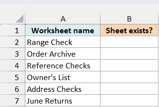
Enter the below formula in B2, then copy it down to B7:
=ISREF(INDIRECT("'"&SUBSTITUTE(A2,"'","''")&"'!A1"))
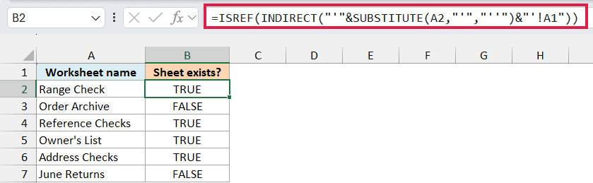
Range Check, Reference Checks, Owner’s List, and Address Checks return TRUE because those tabs exist in the example workbook. Order Archive and June Returns return FALSE because they don’t exist.
Here is how the formula works:
- The SUBSTITUTE function replaces any apostrophe in the sheet name with two apostrophes, which is how Excel handles an apostrophe inside a quoted sheet reference.
- The ampersands join that name to the surrounding single quotes and !A1. For Range Check, the text becomes
'Range Check'!A1. - INDIRECT tries to resolve that text as a reference, and ISREF returns TRUE when it succeeds.
The surrounding quotes allow sheet names with spaces. Doubling the apostrophe also lets the formula handle Owner’s List, which would otherwise break the constructed reference.
A1 is just a cell we can refer to on any worksheet. It doesn’t need to contain anything for the sheet check to return TRUE.
This formula checks the current workbook, and it has the same INDIRECT volatility as the previous example. If you adapt it to another workbook, that workbook must be open for INDIRECT to resolve the reference.
So these are four ways to use ISREF, from checking a cell reference to checking worksheet names stored as text. I hope you found this tutorial useful.
Other Excel Articles You May Also Like:
