

If you want to find the second highest, third highest, or any Nth highest number in a list, MAX won’t get you there because it only ever returns the single biggest value.
The LARGE function is what you need instead. It hands you the value at whatever rank you ask for.
In this article, I’ll show you how to use LARGE to pull the top values from a list, build a spilling top-N list, add up the top few numbers, find the largest value in a category, and handle the errors that trip people up.
Follow along with the example file
LARGE Function Examples.xlsx
When to Use the Excel LARGE Function
Use LARGE when you need a value based on its rank, not just the single biggest one. It returns the Kth largest value from a range, so you pick the position you want.
Say you have a column of sales numbers. MAX gives you the top figure and nothing else. LARGE lets you ask for the 1st, 2nd, 3rd, or any position down the list.
Syntax of the LARGE Function
=LARGE(array, k)
Array – the range or array of numbers you want to pull a value from.
K – the position from the top that you want. K of 1 returns the largest value, 2 returns the second largest, and so on.
A couple of things worth knowing before we get into examples:
- LARGE ignores empty cells, text, and logical values in the range. It only looks at numbers.
- If K is 0 or less, or bigger than how many numbers you have, LARGE returns a #NUM! error.
Example 1: Get the Top 3 Values as a Spilling List
Let’s start with the example most people actually want. You have a list and you want the top few values pulled out in one shot.
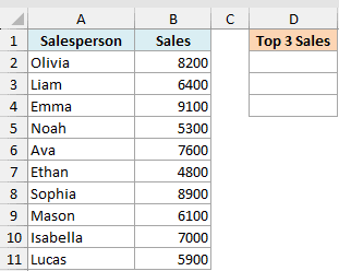
Below is a list of salespeople in column A and their sales for the month in column B. I want the three highest sales figures listed out in column D.
Here is the formula:
=LARGE(B2:B11, SEQUENCE(3))
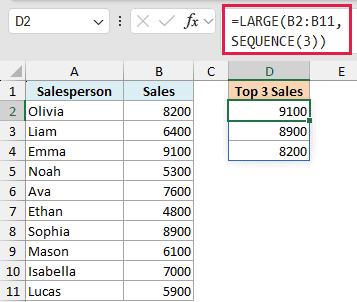
SEQUENCE(3) creates the list of positions {1; 2; 3}, and LARGE returns a value for each one. So you get the 1st, 2nd, and 3rd largest sales figures.
The result spills down automatically. You type the formula once in the top cell and Excel fills the cells below it. No dragging, and no need to press Ctrl + Shift + Enter.
Want the top 5 instead of the top 3? Just change SEQUENCE(3) to SEQUENCE(5) and the list grows on its own.
Pro Tip: SEQUENCE and spilling formulas need Microsoft 365 or Excel 2021. On Excel 2019 or earlier, use the single-K version in the next section and copy it down for each position.
Example 2: Find the Second or Third Largest Value
If you only want one specific position, you can hand LARGE a plain number for K instead of a SEQUENCE.
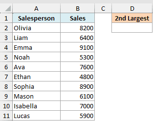
Using the same list of salespeople and sales in A2:B11, here I want the second highest sales figure on its own.
Here is the formula for the second largest value:
=LARGE(B2:B11, 2)
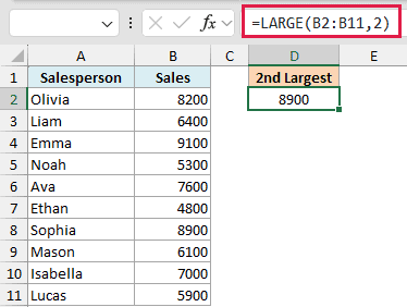
Since K is 2, LARGE skips the top value and returns the one right below it.
For the third largest, change K to 3:
=LARGE(B2:B11, 3)
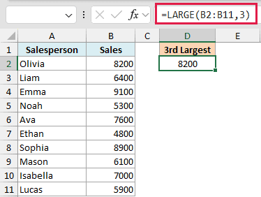
This is the version to reach for on older Excel that doesn’t support spilling. Type the formula once, then copy it down and bump K by hand for each row.
Example 3: LARGE vs MAX: What’s the Difference?
People often mix these two up, so here is the short version. MAX only ever gives you the single largest value. LARGE gives you the value at any rank you name.
Using the same sales list in B2:B11, MAX returns 9100, the same top figure you’d get from =LARGE(B2:B11, 1):
=MAX(B2:B11)
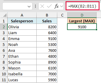
For a range containing numbers, MAX and LARGE with K set to 1 return the same value. With no numbers, MAX returns 0 and LARGE returns #NUM!. The moment you need the 2nd, 3rd, or Nth value, MAX can’t help and LARGE can.
Follow along with the example file
LARGE Function Examples.xlsx
Example 4: Sum the Top 3 Values
A common follow-up question is “what do my top few numbers add up to?” You can nest LARGE inside SUM to total the top values without a helper column.
With the same salespeople and sales in A2:B11, here I want the combined total of the three highest sales figures.
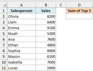
Here is the formula:
=SUM(LARGE(B2:B11, SEQUENCE(3)))
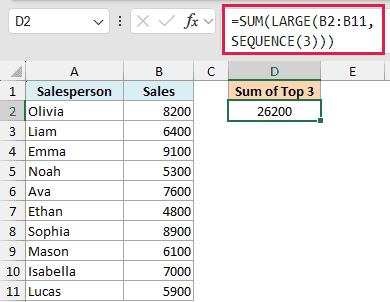
LARGE returns the top three values as a small array, and SUM adds them together in the same cell. Change SEQUENCE(3) to SEQUENCE(5) to total the top five instead.
Pro Tip: On Excel 2019 or earlier, use =SUM(LARGE(B2:B11,{1;2;3})) instead. The hard-typed array {1;2;3} does the same job as SEQUENCE and works without dynamic arrays.
Example 5: Find the Largest Value in a Category (LARGE IF)
There is no LARGEIF function, but you can still get the largest value for a specific category by feeding LARGE a filtered range.
Here I have salespeople in column A, their region in column B, and their sales in column C. I want the highest sales figure for the East region only.
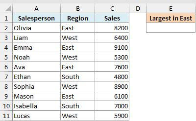
Here is the formula:
=LARGE(FILTER(C2:C11, B2:B11="East"), 1)
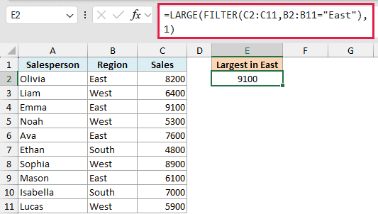
FILTER first pulls out only the sales where the region is East, and LARGE then returns the largest value from that shorter list. Change K to 2 to get the second highest East figure instead.
For just the largest value in a category, MAXIFS is simpler in Microsoft 365 or Excel 2019 and later.
Pro Tip: FILTER needs Microsoft 365 or Excel 2021. On older versions, use =LARGE(IF(B2:B11=”East”,C2:C11),1) and confirm it with Ctrl + Shift + Enter so it runs as an array formula.
Example 6: How LARGE Handles Duplicates
LARGE counts duplicate values as separate positions, which surprises people the first time they see it. It does not skip repeats.
Below I have a short list of scores in A2:A6, and two of them are tied at 92.
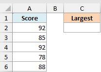
Here is the formula for the largest value:
=LARGE(A2:A6, 1)
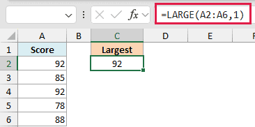
This returns 92. Now here is the second largest:
=LARGE(A2:A6, 2)
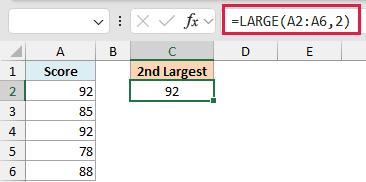
This also returns 92, because LARGE treats the two tied scores as position 1 and position 2. So a value can show up more than once across ranks, and LARGE won’t collapse the ties into a single spot.
Example 7: Handle the #NUM! Error When K Is Too Big
If you ask LARGE for a position that doesn’t exist, you get a #NUM! error. This happens when K is bigger than how many numbers you have, or when K is 0 or a negative number.
Below I have five sales figures in A2:A6, and here I’m asking for the 8th largest value, which doesn’t exist.
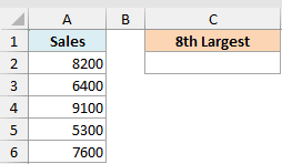
Here is the formula, wrapped in IFERROR to show a friendly message instead of the error:
=IFERROR(LARGE(A2:A6, 8), "Not enough values")
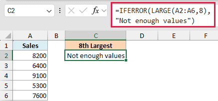
LARGE tries to return the 8th largest value, finds only five numbers, and errors out. IFERROR catches that and shows your text instead.
This is handy when K comes from a cell a user can change, so a too-big number never leaves a raw #NUM! on the sheet. IFERROR catches every error, though, so this message doesn’t always mean there aren’t enough values.
Things to Keep in Mind
- LARGE only looks at numbers. Empty cells, text, and TRUE/FALSE values in the range are ignored, so they never count toward a position.
- Use a whole number for K, from 1 up to the count of numbers in your range. Values below 1 or above that count give a #NUM! error.
- Duplicates each take their own rank. Two values of 92 fill positions 1 and 2. They don’t share a single spot.
- SMALL is the mirror image of LARGE. For the smallest, second smallest, and so on, use the SMALL function the same way you use LARGE here.
- Pulling the top and bottom few values is also a quick way to spot outliers. Extract the largest and smallest handful with LARGE and SMALL, then eyeball them. There’s a full walkthrough in how to find outliers in Excel.
That covers the main ways to use the LARGE function in Excel, from pulling a single Nth value to spilling the whole top N and totaling it in one formula.
Once you’re comfortable asking for a value by its rank, a lot of “top performers” style reports get much quicker to build. I hope you found this article helpful.
Excel LARGE Function – Video Tutorial
Other Excel Articles You May Also Like:
