RANK Function in Excel (6 Examples)

If you want to rank a list of numbers in Excel, say the highest sales figure as rank 1, the next as rank 2, and so on, you don’t have to sort the data or count positions by hand.

The RANK function does this for you, and it works in every version of Excel. In Excel 365, you can also give RANK the entire range at once and the ranks spill into the cells below.

In this article, I’ll show you how to use the RANK function to rank numbers from highest to lowest, from lowest to highest, how it treats tied values, and how to get unique ranks or rank within groups.

RANK Function Syntax

Here is the syntax of the RANK function:

=RANK(number, ref, [order])

• number – the number you want to rank.
• ref – the list of numbers you’re ranking the number against. This is usually a range of cells.
• [order] – optional. Use 0 (or leave it out) to rank from highest to lowest. Use 1 to rank from lowest to highest.

Pro Tip: Excel 2010 added RANK.EQ and RANK.AVG as newer versions of RANK, and the old RANK function is kept for backward compatibility. RANK.EQ gives exactly the same results as RANK, so everything in this tutorial applies to it too. RANK still works fine in all versions, including Excel 365.

When to Use the RANK Function in Excel

Use the RANK function when you need to:

• Find the position of a value in a list, like the third-highest sales figure or the fastest response time
• Rank scores, sales, or totals without sorting the data
• Build leaderboards that update automatically as the numbers change
• Spot the top and bottom performers in a dataset at a glance

Let me show you a few practical examples of how to use the RANK function.

Example 1: Rank Numbers From Highest to Lowest

Let’s start with the most common case, ranking values so the biggest number gets rank 1.

Below I have a dataset with ten retail stores in column A and their monthly sales in column B. Column C is where the ranks will go.

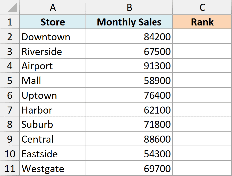
I want to rank the stores by sales, so the store with the highest sales gets rank 1.

Here is the formula for cell C2:

=RANK(B2,$B$2:$B$11)

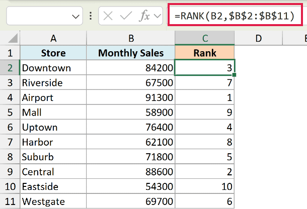
This ranks the sales figure in B2 against the whole list in B2:B11. I left out the third argument, so RANK uses the default order and the biggest number becomes rank 1.

Notice the dollar signs in $B$2:$B$11. That locks the range so it stays fixed when you copy the formula down. The B2 part has no dollar signs, so it moves to B3, B4, and so on for each row.

Once you enter the formula in C2, copy it down for the rest of the rows to rank all the stores.

Example 2: Rank a Whole Column with One Formula (Excel 365)

If you’re on Excel 365, you don’t even need to copy the formula down. One formula can rank the entire list.

I’m using the same dataset here, with ten stores in column A and their monthly sales in column B.

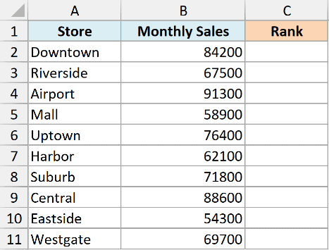
I want all ten ranks from a single formula in cell C2.

Here is the formula:

=RANK(B2:B11,B2:B11)

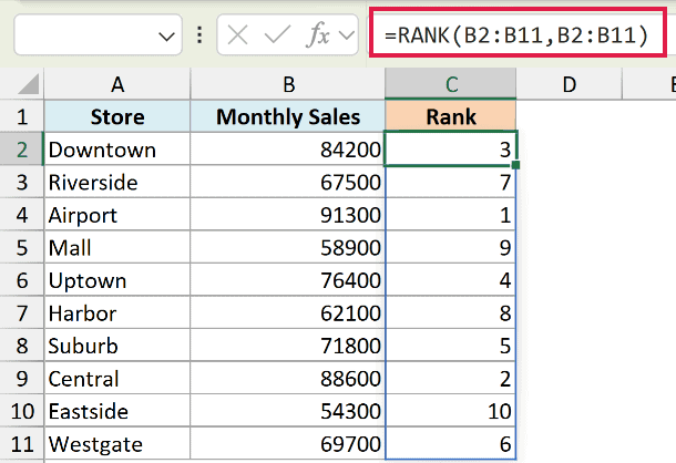
Because the first argument is the whole range instead of a single cell, RANK returns one rank for every value and spills the results down column C automatically.

You don’t copy anything down, and since the same range is used for both arguments, you don’t need the dollar signs either.

Pro Tip: Spilling formulas need the cells below the formula to be empty. If C3:C11 already have something in them, you’ll get a #SPILL! error instead of the ranks.

Example 3: Rank From Lowest to Highest

Sometimes you want the smallest value to be rank 1. Lower is better for things like delivery times, error counts, or expenses.

Below I have a dataset with eight customer support agents in column A and their average first-response time in hours in column B.

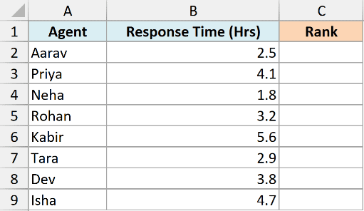
I want to rank the agents so the fastest one, the one with the lowest response time, gets rank 1.

Here is the formula for cell C2:

=RANK(B2,$B$2:$B$9,1)

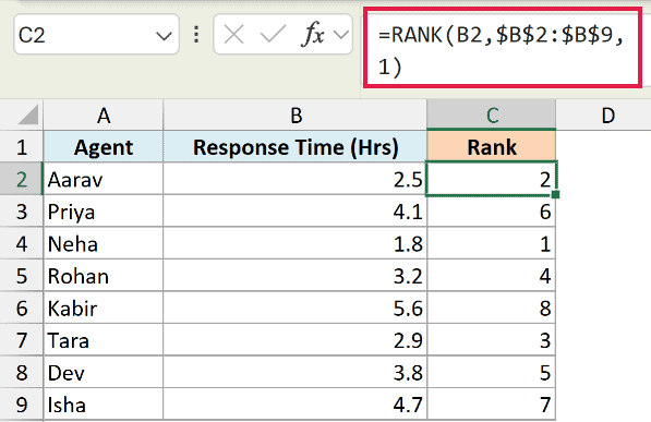
The 1 as the third argument flips the direction. Now the smallest number gets rank 1 and the largest gets the highest rank.

Everything else works the same as before. The range is locked with $B$2:$B$9, and you copy the formula down the column.

Example 4: How RANK Handles Tied Values

When two or more numbers in the list are the same, RANK gives them all the same rank and then skips the next rank(s). Let me show you what that looks like.

Below I have a dataset with eight products in column A and the units sold for each in column B. Three products sold 620 units and two sold 480, so there are ties.

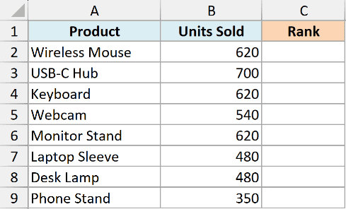
I want to rank the products by units sold, highest first, and see what RANK does with the duplicates.

Here is the formula for cell C2:

=RANK(B2,$B$2:$B$9)

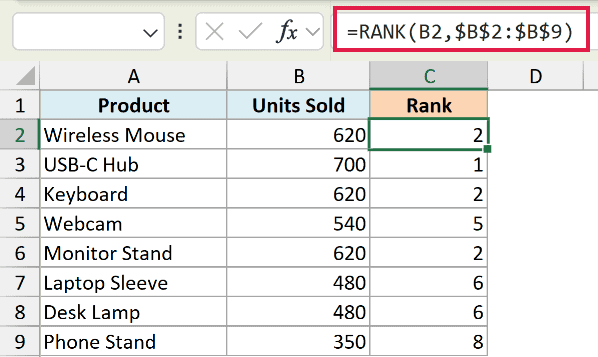
The three products that sold 620 units all get rank 2. RANK then skips ranks 3 and 4, so the next product down lands at rank 5.

The same thing happens with the two products at 480 units. Both get rank 6, rank 7 is skipped, and the last product gets rank 8.

This is expected behavior, not an error. It matches the everyday idea of “joint second place” in a competition.

Pro Tip: If you’d rather give tied values the average of the ranks they occupy (so the three-way tie above shows 3 instead of 2), use the RANK.AVG function. It takes the same arguments as RANK.

Example 5: Give Every Number a Unique Rank

RANK repeats ranks when values tie. Sometimes you need a clean list where every number has its own rank, with no repeats and no gaps.

I’m using the same dataset as the last example, eight products in column A and their units sold in column B, including the tied values.

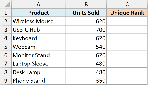
I want a unique rank for every product in column C, even for the ones that sold the same number of units.

Here is the formula for cell C2:

=RANK(B2,$B$2:$B$9)+COUNTIF($B$2:B2,B2)-1

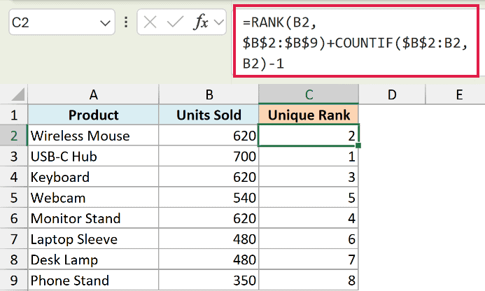
How this formula works:

• RANK(B2,$B$2:$B$9) gives the normal rank, which repeats for tied values.
• COUNTIF($B$2:B2,B2) counts how many times the current value has appeared from the top of the list down to this row. The first tied value gets 1, the second gets 2, and so on.
• Subtracting 1 keeps the first occurrence at its original rank, then nudges each later tie down by one.

The result is a ranking that runs 1, 2, 3, and so on with no repeats. Ties are broken by which row comes first, so the product higher up in the list keeps the better rank.

Note the range trick in the COUNTIF part. The first cell $B$2 is locked, but the second B2 is not.

As you copy the formula down, that range grows from $B$2:B2 to $B$2:B3, $B$2:B4, and so on. That’s what lets it count only the ties seen so far.

Example 6: Rank Within Groups or Categories

Often you don’t want one overall ranking. You want to rank each item inside its own group, like ranking salespeople within their region.

Below I have a dataset with salespeople in column A, their region in column B, and their sales in column C. The rows are a mix of East, West, and North regions.

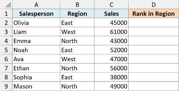
I want to rank each person against only the others in the same region, so every region has its own rank 1.

RANK can’t limit itself to one group, so we use COUNTIFS instead. Here is the formula for cell D2:

=COUNTIFS($B$2:$B$9,B2,$C$2:$C$9,">"&C2)+1

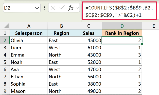
How this formula works:

• $B$2:$B$9,B2 limits the count to rows in the same region as the current row.
• $C$2:$C$9,">"&C2 counts how many people in that region have higher sales than the current person.
• Adding 1 turns that count into a rank, so the top seller in each region has zero people above them and lands at rank 1.

Copy the formula down and each person gets ranked only against others in their own region. Switch the > to < if you’d rather rank from lowest to highest inside each group.

Tips and Common Mistakes

A few things that trip people up with the RANK function:

• Lock the range with dollar signs. When you copy a rank formula down, the list you rank against must stay fixed. Use $B$2:$B$11, not B2:B11, or the range will shift and the ranks will be wrong.
• RANK skips ranks after a tie. If two values tie for rank 2, the next value is rank 4, not 3. That’s expected behavior. Use the COUNTIF method above if you need a gap-free list.
• Text and blank cells are ignored. RANK works on numbers only. Empty cells and text in the range are skipped, so they won’t throw off your ranking.
• The number should be in the list. If the number you’re ranking isn’t found in ref at all, RANK returns a #N/A error.
• Getting the direction wrong. Forgetting the third argument when ranking times or costs puts the worst value at rank 1. Use 1 whenever a smaller number should win.

That’s how the RANK function works in Excel. Rank from highest to lowest by default, pass 1 to flip the direction, and add COUNTIF or COUNTIFS when you want unique ranks or ranking within groups.

I hope you found this tutorial useful.

List of All Excel Functions

Other Excel Articles You May Also Like:

• How to Use Excel LARGE Function
• SMALL Function in Excel
• Find the Second Largest Value in Excel
• Automatically Sort Data in Alphabetical Order using Formula