

If you want to count how many cells in a range meet a condition, such as how many times an item shows up or how many values cross a limit, the COUNTIF function does exactly this.
COUNTIF returns a single value, but it also works inside dynamic array formulas. Pair it with UNIQUE and one formula can count every category in your data at once (I show this in Example 8).
In this article, I’ll show you how to use COUNTIF in Excel with text, numbers, wildcards, blank cells, and dates.
Follow along with the example file
COUNTIF Function Examples.xlsx
COUNTIF Function Syntax
Here is the syntax of the COUNTIF function:
=COUNTIF(range, criteria)
- range – The group of cells you want to check. This can be a column, a row, or any block of cells.
- criteria – The condition a cell must meet to be counted. It can be a number, text, a comparison like “>30”, or a cell reference.
That’s it. Two arguments, and only the cells in the range that meet the criteria get counted.
Pro Tip: COUNTIF checks only one condition. If you need to count based on two or more conditions, use the COUNTIFS function instead.
When to Use COUNTIF in Excel
Use the COUNTIF function when you need to:
- Count how many times a specific name, product, or entry appears in a list
- Count values above or below a number
- Count cells that contain any text, or a specific word, using wildcards
- Count blank cells in a column
- Count dates before or after a cutoff date
Let me show you a few practical examples of how to use this function.
Example 1: Count Cells With a Specific Text Value
Let’s start with a simple example.
Below is a dataset with office equipment sales, where I have the item names in column A and the quantity sold in column B.
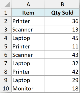
I want to count how many times Printer appears in column A.
Here is the formula:
=COUNTIF(A2:A10,"Printer")
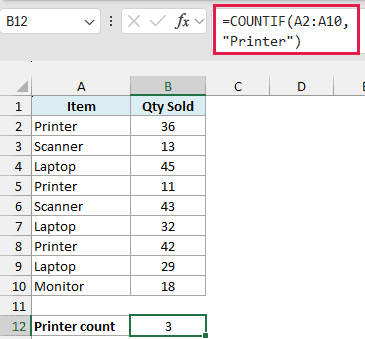
This returns 3, since Printer shows up three times in the list.
Excel goes down the range A2:A10 and counts every cell that says Printer. The text criteria is wrapped in double quotes, and it’s not case-sensitive, so “printer” or “PRINTER” would give the same count.
Example 2: COUNTIF With a Cell Reference as the Criteria
Instead of typing the criteria into the formula, you can keep it in a cell and refer to that cell. This way you can change the criteria without touching the formula.
Below is a dataset with IT support requests, where I have the requesting department for each ticket in column A. Cell D2 has the department I want to count (HR).
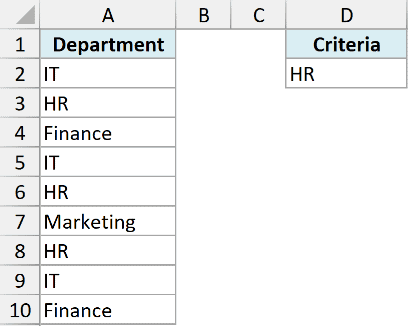
I want to count how many requests came from the department entered in cell D2.
Here is the formula:
=COUNTIF(A2:A10,D2)
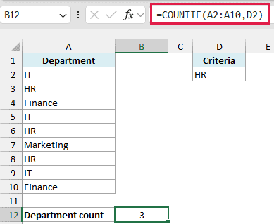
This returns 3, the number of HR requests.
The criteria is now whatever sits in D2. Type Finance or IT in that cell and the count updates on its own. Note that a cell reference used as criteria does not need quotes.
Example 3: COUNTIF Greater Than a Value
Just like text, COUNTIF works with numbers, and the criteria can be a comparison.
Below is a dataset with kitchen appliance sales, where I have the product names in column A and the units sold in column B.
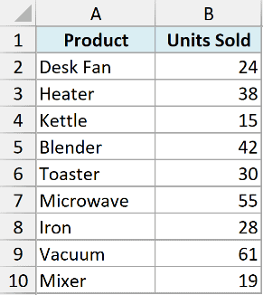
I want to count how many products sold more than 30 units.
Here is the formula:
=COUNTIF(B2:B10,">30")
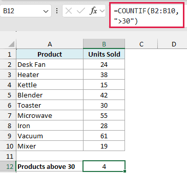
This returns 4, the number of products with sales above 30.
The operator and the number go together inside double quotes. A product that sold exactly 30 units is not counted, since the check is strictly greater than. Use “>=30” if you want to include it.
The same pattern works with other operators too, such as “<” to count cells less than a value or “<>” for not equal to. And if the limit sits in a cell, join the operator and the reference with an ampersand, like “>”&D2.
Follow along with the example file
COUNTIF Function Examples.xlsx
Example 4: Count Cells That Contain Any Text
Here’s a handy one. Excel has the COUNT function for cells with numbers, but there is no built-in function that counts only the text cells. COUNTIF fills that gap.
Below is a dataset with a messy imported column, where column A has a mix of text codes and numbers.
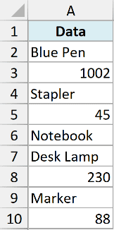
I want to count only the cells that contain text and ignore the numbers.
Here is the formula:
=COUNTIF(A2:A10,"*")
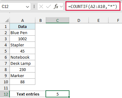
This returns 5, the number of text entries.
The asterisk (*) is a wildcard character that represents text of any length. Numbers and truly empty cells don’t match it. A formula returning an empty string does match, so it is included in the count.
Pro Tip: The COUNTA function counts all non-empty cells (text and numbers), and COUNT counts only numbers. COUNTIF with “*” is the one that isolates text.
Example 5: Count Cells That Contain a Specific Word
You can also combine wildcards with a word to count partial matches.
Below is a dataset with employee job titles in column A. Some titles include the word Manager and some don’t.
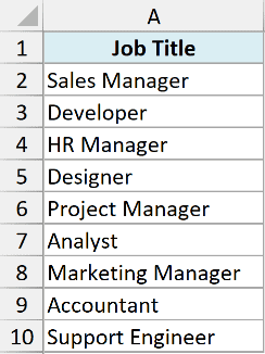
I want to count how many job titles contain the word Manager anywhere in the text.
Here is the formula:
=COUNTIF(A2:A10,"*Manager*")
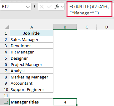
This returns 4, the number of titles with Manager in them.
An asterisk on each side of the word means “Manager can appear anywhere in the cell”. There is also the question mark (?) wildcard, which matches exactly one character. I’ve covered more patterns like these in my guide on counting cells that contain text strings.
Pro Tip: To count cells whose entire value is an actual asterisk or question mark, put a tilde before it. For example, use “~*” in the criteria to match a real asterisk instead of treating it as a wildcard.
Example 6: Count Blank Cells
Here’s a scenario I run into all the time, checking who hasn’t responded yet.
Below is a dataset with a wedding RSVP tracker, where I have the guest names in column A and their responses in column B. Some guests haven’t replied, so their response cells are empty.
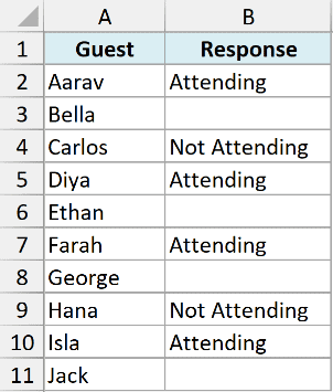
I want to count how many guests haven’t replied yet, which means counting the blank cells.
Here is the formula:
=COUNTIF(B2:B11,"")
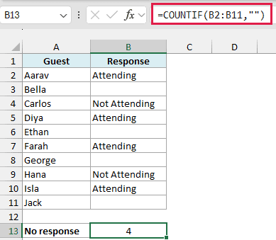
This returns 4, the number of guests with no response.
Two double quotes with nothing between them mean “an empty cell”. The COUNTBLANK function does the same job if you prefer a dedicated function. And to flip it around and count the cells that are filled, use “<>” as the criteria.
Example 7: COUNTIF With Dates
Let’s use dates as the criteria now.
Below is a dataset with driving test bookings, where I have the student names in column A and their test dates in column B.
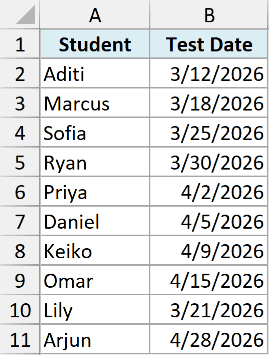
I want to count how many tests are scheduled on or after April 1, 2026.
Here is the formula:
=COUNTIF(B2:B11,">="&DATE(2026,4,1))
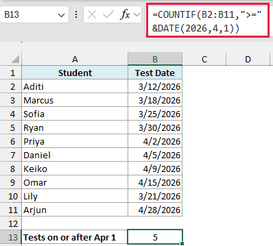
This returns 5, the number of tests on or after April 1, 2026.
The DATE function builds the date inside the formula, so it works no matter which regional date format your system uses. The ampersand joins the “>=” operator to that date, the same pattern you’d use with a cell reference.
Pro Tip: To count dates from today onward, use “>=”&TODAY() as the criteria. The count then updates when the workbook recalculates.
Example 8: Count Each Unique Value With One Formula
This last one is my favorite, and it’s something most COUNTIF tutorials skip.
Below is a dataset with podcast episodes, where I have the episode numbers in column A and the topic each episode covers in column B. Topics repeat across episodes, and I’ve set up a small summary area with Topic and Episodes headers in columns D and E.
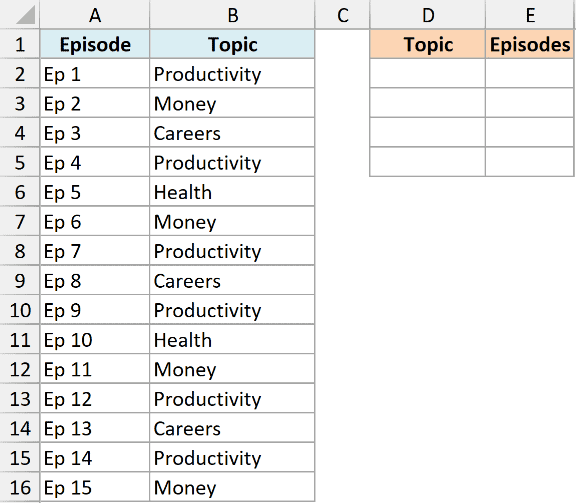
I want a summary that lists each topic once, with a count of how many episodes cover it.
First, I get the list of topics with the UNIQUE function in cell D2:
=UNIQUE(B2:B16)
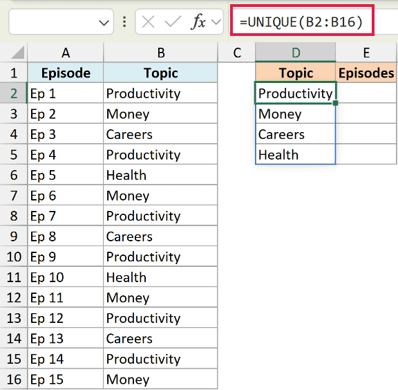
UNIQUE is a dynamic array function, so this single formula spills all four distinct topics into the cells below D2.
Now comes the trick. In cell E2, I point COUNTIF at that spilled list using the hash (#) reference:
=COUNTIF(B2:B16,D2#)
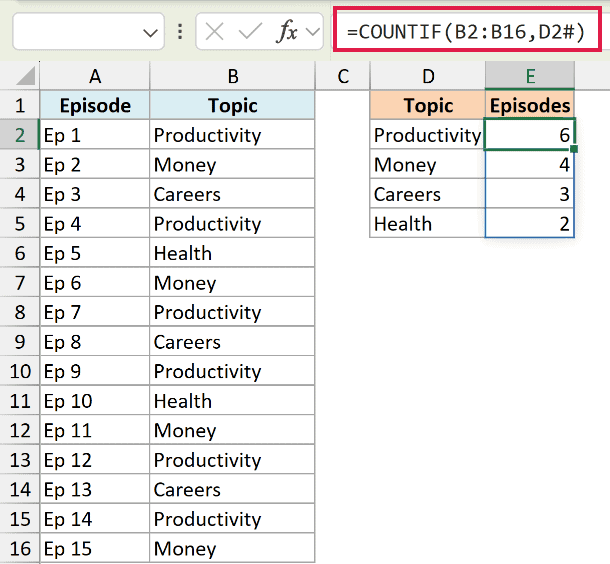
This single formula spills a count next to every topic. D2# means “the entire range that spills from D2”, so COUNTIF takes each topic as a criteria and returns all the counts in one go.
You don’t need to fill anything down or fix any ranges. If a new episode adds a fifth topic, extend the ranges and the whole summary rebuilds itself.
You’ll need Excel 365 or Excel 2021 for this example, since UNIQUE and spilled ranges aren’t available in older versions.
Tips & Common Mistakes
- Quotes trip people up the most. Text and comparison criteria need double quotes (“Printer”, “>30”), but a plain number doesn’t, so =COUNTIF(B2:B10,30) is fine.
- COUNTIF is not case-sensitive. “printer” and “Printer” are the same to it. If you need a case-sensitive count, use SUMPRODUCT with the EXACT function.
- Only one condition per COUNTIF. Use COUNTIFS when every condition must match. Adding COUNTIF results works for OR conditions only when they don’t overlap; otherwise a cell can be counted twice. I’ve covered both routes in using multiple criteria in COUNTIF.
- COUNTIF can’t count by cell color. The criteria only checks values, not formatting. To count colored cells, you need a workaround like SUBTOTAL with a filter or VBA.
- Watch for extra spaces. A trailing space makes “Printer ” different from “Printer”, so the count comes up short. Clean the data with TRIM if the counts look off.
- The range must be an actual range on the sheet. You can’t feed COUNTIF an array from another function as its range argument. The criteria argument, though, happily accepts a spilled range like D2# (as you saw in Example 8).
- Long text can miscount. COUNTIF gives incorrect results when matching strings longer than 255 characters.
COUNTIF is one of those functions you end up using in almost every workbook, whether it’s a quick sanity check on a list or a full summary table. Master the criteria patterns in these examples (exact match, operators, wildcards, blanks, and dates) and you’re covered for nearly every counting job in Excel.
I hope you found this article helpful.
Other Excel Articles You May Also Like:
- Count Between Two Numbers in Excel (COUNTIF / COUNTIFS)
- Count Unique Values in Excel Using COUNTIF Function
- How to Use Excel COUNT Function
- Count Characters in a Cell (or Range of Cells) in Excel
- Count Cells That Are Not Blank in Excel
- Create a Yes/No Drop-Down List in Excel
- AVERAGEIF Function in Excel
- ISBLANK
