

The LOGEST function in Excel fits an exponential curve to your data and returns the numbers that describe that curve. It’s useful when values grow or shrink by a roughly steady percentage, such as 10% per month.
You get a growth factor and a starting value, which you can use to describe the pattern or estimate another value. LOGEST can also return statistics that help you judge how closely the curve fits your observations.
In this tutorial, I’ll show you five examples, including growth, forecasting, decay, and a model with two inputs.
Follow along with the example file
LOGEST Function Examples.xlsx
LOGEST Function Syntax
Here is the syntax of the LOGEST function:
=LOGEST(known_y's, [known_x's], [const], [stats])
- known_y’s is required. These are the observed values you want to model, such as the number of downloads each week.
- known_x’s is optional. These are the matching input values, such as week numbers. You can supply one input variable or several; if omitted, Excel uses 1, 2, 3, and so on.
- const is optional. TRUE, or leaving it out, lets Excel estimate the starting value
b. FALSE fixesbat 1 and fits the other coefficients around that restriction. - stats is optional. FALSE, or leaving it out, returns only the coefficients. TRUE adds four rows of regression statistics below them.
For one input variable, the x and y ranges must have the same dimensions. With several input variables, keep the y values in a single column and give each input its own column with the same number of rows.
You can also arrange the data across rows. In that case, keep the y values in one row and put each input variable in a separate matching row.
Setting const to FALSE means the fitted value is 1 when every x value is zero. It does not mean the starting value is zero, so leave this argument TRUE unless your model genuinely requires that restriction.
LOGEST works in Excel 365, 2024, 2021, 2019, and 2016. In Excel 365, 2024, and 2021, press Enter to spill the results; in Excel 2019 or earlier, select the output range first and confirm with Ctrl+Shift+Enter.
When to Use the LOGEST Function
Use LOGEST when you need to:
- Estimate the percentage growth or decline that best fits a set of observations.
- Get the coefficients of an exponential model so you can use them in other calculations.
- Examine an exponential model’s regression statistics.
- Fit an exponential model with more than one input variable.
An exponential model assumes the same multiplicative change for each one-unit increase in an input. For example, multiplying by 1.10 each month means 10% monthly growth, even though the number added gets larger over time.
If your data changes by a roughly fixed amount instead, a straight-line model is more appropriate. The LINEST function returns the coefficients for that model.
Let me show you how LOGEST works with a small dataset.
Example 1: Find Exponential Growth with LOGEST
Below are eight weeks of recipe-download counts, and we want the fitted growth factor and starting value in columns D and E.
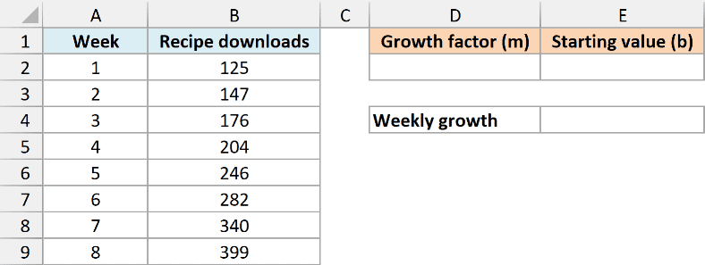
On the Growth sheet, enter this formula in cell D2:
=LOGEST(B2:B9,A2:A9)
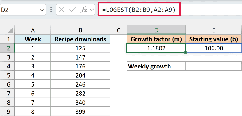
The formula uses the download counts as y values and the week numbers as x values. It returns two coefficients across D2:E2: approximately 1.1802 and 106.00.
These belong to the equation y = b * m^x, where ^ means “raised to the power of.” LOGEST returns m first and b second.
Here, m is the factor applied for each additional week. A factor of 1.1802 means the fitted count becomes about 1.1802 times as large each week.
The second number, b, is the model’s value at week zero. It’s about 106, even though the first observed count is 125, because our observations start at week one.
To express the growth factor as a percentage, enter this formula in E4 and format the cell as Percentage with two decimal places:
=D2-1
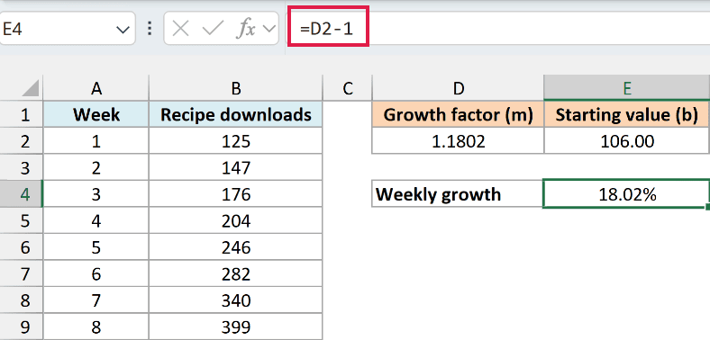
The result is 18.02%. That’s the constant weekly growth rate fitted across all eight observations, so individual weeks don’t have to grow by exactly that percentage.
Because these week numbers are 1 through 8, leaving out the second argument would give the same coefficients. Keep the x range when your sequence starts at zero or has gaps, or Excel will fit a different set of x values.
Make sure the two output cells are empty before entering LOGEST. If another value blocks the second cell, Excel shows #SPILL! instead of the two coefficients; clear the obstruction and keep the formula in the left cell.
Important: Every numeric y value must be greater than zero. A zero or negative count produces #NUM! because LOGEST fits the natural logarithms of those values; don’t replace genuine zeros with invented positive numbers to force a result.
If you’re using Excel 2019 or earlier, select D2:E2 on the Growth sheet, enter the formula below, and press Ctrl+Shift+Enter. Selecting both cells matters because the output includes both coefficients.
=LOGEST(B2:B9,A2:A9)
Example 2: Forecast Using the Fitted Curve
Once you have the coefficients, you can use them to estimate another point on the curve.
Below is the Forecast sheet with the same weekly downloads and fitted coefficients, and we want the predicted count for week 9 in cell E5.
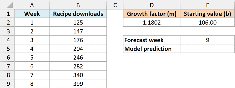
The forecast week is in E4. Enter this formula in E5:
=E2*D2^E4
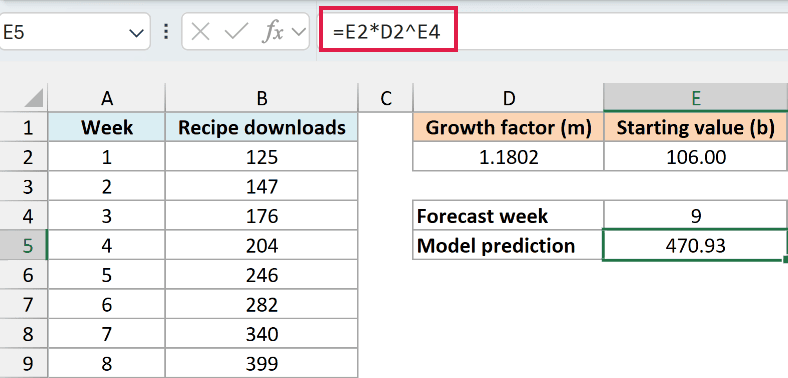
This uses b * m^x: E2 contains the starting value, D2 contains the growth factor, and E4 contains the week number. The result is 470.93, or about 471 downloads.
Referencing the coefficient cells keeps Excel’s full precision. Typing the rounded numbers shown in the screenshot into the prediction formula would give a slightly different result.
If you only need a prediction, the GROWTH function can fit the curve and return that prediction in one formula. Enter this in E6 to compare the result:
=GROWTH(B2:B9,A2:A9,E4)
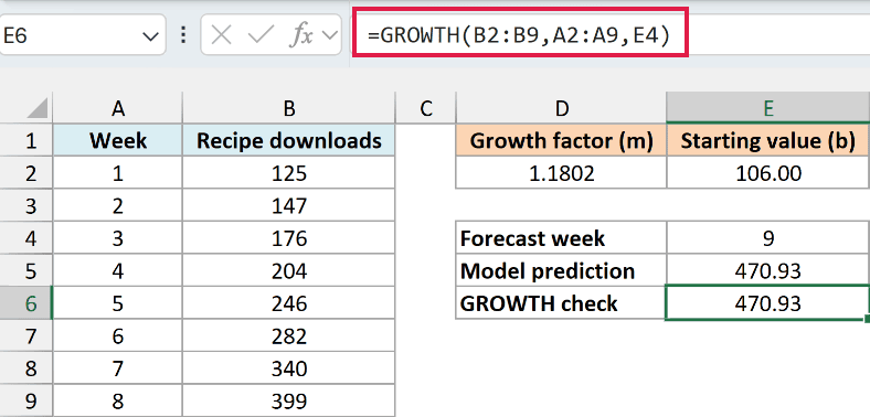
It also returns 470.93. Use the coefficient calculation when you already have m and b; use GROWTH when you don’t need to inspect those coefficients.
Week 9 is outside the observed weeks, so this prediction assumes the existing growth pattern continues. A good historical fit doesn’t guarantee that next week’s downloads will follow it.
Example 3: Measure Exponential Decay
LOGEST also handles values that decrease over time. The fitted factor will be between zero and one.
Below are the unsold tickets remaining during eight days of an event sale, and we want the daily factor and starting estimate in columns D and E.
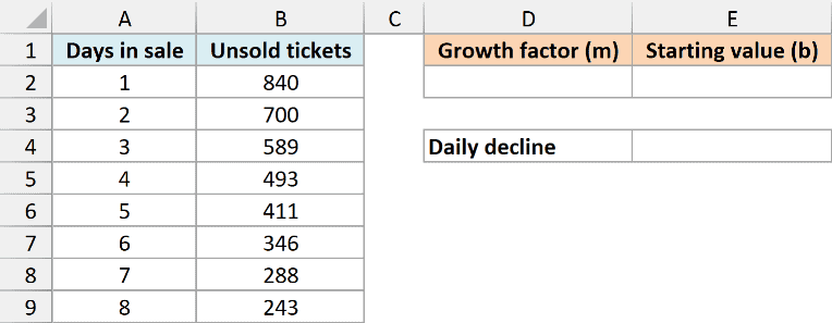
On the Decay sheet, enter this formula in D2:
=LOGEST(B2:B9,A2:A9)
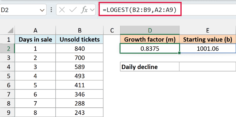
The factor is approximately 0.8375, with an estimated starting value of 1,001.06. The model says that about 83.75% of the previous day’s unsold tickets remain after each additional day.
To show the daily decline as a positive percentage, enter this formula in E4 and format it as Percentage with two decimal places:
=1-D2
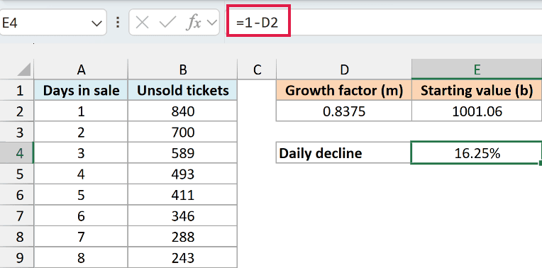
The result is 16.25%. This describes the fitted rate of decline in unsold tickets, not a fixed number of tickets sold each day.
A factor above one indicates growth, a factor below one indicates decay, and a factor of one indicates no fitted change. The header still calls it a growth factor because it’s the same m coefficient in each case.
Follow along with the example file
LOGEST Function Examples.xlsx
Example 4: Read the LOGEST Regression Statistics
The coefficients describe the curve, but they don’t tell you how closely the observations follow it. The stats argument gives you additional information about the fit.
Below are the recipe-download counts on the Statistics sheet, and we want the coefficients and regression statistics in columns E and F.
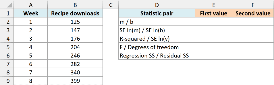
Enter this formula in E2:
=LOGEST(B2:B9,A2:A9,TRUE,TRUE)
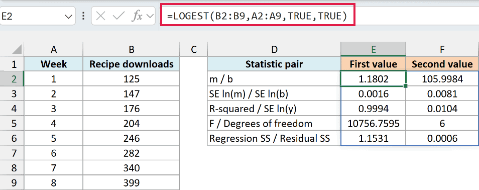
The first TRUE lets Excel estimate b. The second TRUE asks for statistics, so the result fills five rows and two columns, E2:F6.
LOGEST fits a straight line to the natural logarithm of y, written as ln(y), and then converts the first-row coefficients back to m and b. The statistics below that first row still describe the logarithmic fit.
Here is what each row contains:
| Worksheet row | First value in column E | Second value in column F |
|---|---|---|
| 2 | Growth factor m | Starting value b |
| 3 | Standard error of ln(m) | Standard error of ln(b) |
| 4 | R-squared for the log-scale fit | Standard error of the ln(y) estimate |
| 5 | F statistic | Degrees of freedom |
| 6 | Regression sum of squares | Residual sum of squares |
R-squared, in E4, is about 0.9994. For this model, it means the week number explains about 99.94% of the variation in the logarithms of the download counts.
The standard errors describe uncertainty or typical scatter in the logarithmic fit. For example, F4 displays about 0.0104, but that does not mean the predictions are usually off by 0.0104 downloads.
The F statistic compares the variation explained by the fitted relationship with the unexplained variation, after accounting for their degrees of freedom. For LOGEST, this comparison is on the logarithmic scale; its size alone doesn’t prove the model is appropriate.
The residual degrees of freedom are 6 here because there are eight observations and two fitted parameters, the slope and intercept of the logarithmic model. A significance test also needs the predictor degrees of freedom and the regression’s statistical assumptions.
The regression and residual sums of squares split the log-scale variation into the part explained by the model and the part left over. The small residual value here is consistent with the observations sitting close to an exponential curve.
A high R-squared alone doesn’t establish that an exponential model is appropriate or that future forecasts will be accurate. Check the pattern in the data as well, especially before extending it far beyond the observed weeks.
For Excel 2019 or earlier, select E2:F6, enter the formula below, and confirm it with Ctrl+Shift+Enter. A two-cell selection would only show the coefficient row, leaving out the statistics.
=LOGEST(B2:B9,A2:A9,TRUE,TRUE)
Example 5: Use Two Input Variables
You aren’t limited to a single x column. LOGEST can fit an exponential model using several input variables together.
Below are eight sample campaigns with demo hours, email sends, and signups, and we want the fitted coefficients in columns E through G.
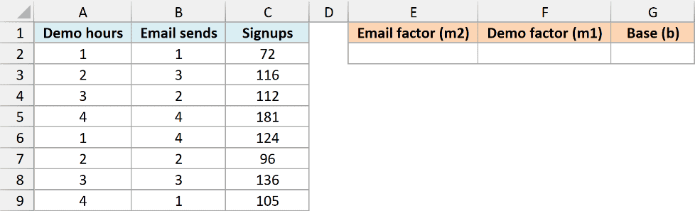
Each row describes one campaign, and Email sends counts how many times an email went to that campaign’s list, not the number of individual recipients. On the Two Predictors sheet, enter this formula in E2:
=LOGEST(C2:C9,A2:B9)
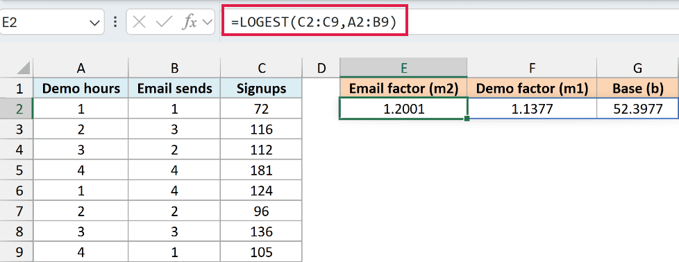
The signup counts are the y values. The two-column x range contains demo hours first and email sends second.
LOGEST returns the coefficients in reverse input-column order, followed by b:
- E2 contains the email-send factor, approximately 1.2001.
- F2 contains the demo-hours factor, approximately 1.1377.
- G2 contains the base value, approximately 52.3977.
The fitted equation is Signups = b * m1^DemoHours * m2^EmailSends. So the factor associated with column A comes from F2, while the factor associated with column B comes from E2.
Within this fitted model, one additional email send multiplies the fitted signup count by about 1.20 while demo hours stay fixed. That is an association in the sample data, not proof that sending an extra email causes that increase.
Keep all input columns aligned with the correct outcome row. Unequal range lengths can return #REF!, while mismatched row ordering can produce plausible-looking coefficients for the wrong relationships.
For Excel 2019 or earlier, select E2:G2, enter the formula below, and confirm it with Ctrl+Shift+Enter to return all three coefficients.
=LOGEST(C2:C9,A2:B9)
These examples show how to read LOGEST’s coefficients, use them in a forecast, and interpret its extra statistics. Keep the units of your x values clear, because a weekly growth factor and a daily growth factor describe different rates.
Other Excel Articles You May Also Like:
