

The TREND function fits a straight line through the numbers you already have and gives you the values that sit on that line. It’s the formula version of adding a trendline to a chart.
You can use it to see the overall direction in data that bounces around, forecast the next few values, or estimate one number from another. In this tutorial, I’ll show you how TREND works with simple examples first, then with two variables and curved data.
Follow along with the example file
TREND Function Examples.xlsx
TREND Function Syntax
Here is the syntax of the TREND function:
=TREND(known_y's, [known_x's], [new_x's], [const])
- known_y’s – the values you already have and want to find the trend for, such as sales, times, or prices. This is the only required argument.
- known_x’s – (optional) the matching values that the y-values depend on, such as week numbers, dates, or distances.
- new_x’s – (optional) the x-values you want TREND to calculate y-values for.
- const – (optional) TRUE or FALSE. If you leave it out, it’s TRUE.
If you leave out known_x’s, Excel uses 1, 2, 3, and so on, one number for each value in known_y’s. So when your data is in order with one row per period (week 1, week 2, and so on), you can skip this argument.
If you leave out new_x’s, TREND uses your known_x’s, so you get one trend value for each value you already have. When you do give new_x’s, you get one result for each new x-value instead.
With const as TRUE, Excel calculates the line’s starting point (the intercept) normally. Setting it to FALSE forces the line to start at zero, which I cover in Example 6.
The TREND function works in all Excel versions, including Excel 365, 2024, 2021, 2019, 2016, Excel for Mac, and Excel for the web.
When to Use the TREND Function
Use this function when you need to:
- See the overall direction in numbers that go up and down
- Forecast the next few weeks or months from past data
- Estimate a value from a related number, such as delivery time from distance
- Predict a value from two or more factors at once
- Find out which values are above or below the trend
Let me show you a few practical examples of how to use the TREND function.
Example 1: Get Trend Values for Your Existing Data
Let’s start with a simple example.
Below is a log of a runner’s 5K time over ten weeks of training, and I want to get the trend time for each week in column C.
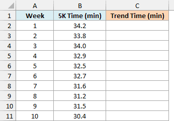
Here is the formula:
=TREND(B2:B11,A2:A11)
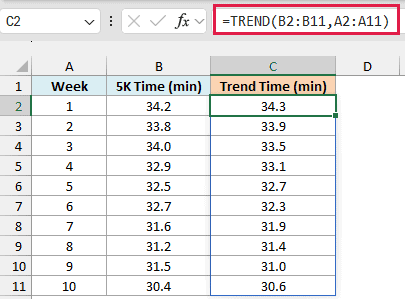
Here, B2:B11 has the 5K times (known_y’s) and A2:A11 has the week numbers (known_x’s). Since I didn’t give any new_x’s, TREND returns the value on the trend line for each of the ten weeks, and the results spill into C2:C11.
The actual times go up and down from week to week, but the trend times drop by about 0.4 minutes every week. That steady drop is the runner’s real improvement, with the good and bad days smoothed out.
This 0.4-minute drop per week is the slope of the trend line, which you can also get on its own with the SLOPE function.
If you are using Excel 2019 or earlier, enter the below formula in cell C2 and then copy it down the range:
=TREND($B$2:$B$11,$A$2:$A$11,A2)
The dollar signs keep the known ranges fixed as you copy, and A2 tells TREND which week to calculate. The same approach works for the other examples in this article if you don’t have dynamic arrays.
Important: TREND needs a number in every cell of known_y’s and known_x’s. A blank cell or a text value in either range returns the #VALUE! error, and ranges of different sizes return the #REF! error.
Example 2: Forecast the Next Few Months With TREND
Now let’s use TREND to look ahead.
Below is a newsletter’s subscriber count for each of the last twelve months, and I want to forecast the subscribers for the next three months in column E.
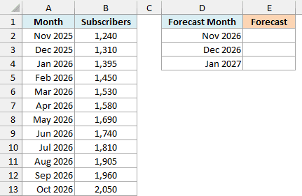
Here is the formula:
=TREND(B2:B13,A2:A13,D2:D4)
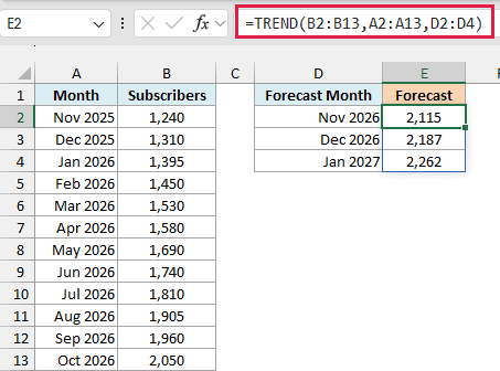
Here, B2:B13 has the subscriber counts, A2:A13 has the months, and D2:D4 has the three future months. TREND fits a line through the twelve months you have, then extends it to give 2,115, 2,187, and 2,262 subscribers for the next three months.
The months in column A are real dates, and that works because Excel stores dates as numbers. So you don’t need a helper column with month numbers 1 to 12.
A straight-line forecast assumes the growth continues at the same pace and can’t follow seasonal ups and downs, so trust it less the further out you go. For seasonal data, other ways to forecast in Excel, such as FORECAST.ETS, work better.
Example 3: Find Which Weeks Beat the Trend
Here’s a different way to use the trend.
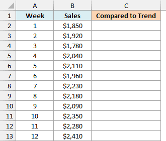
Below are a food truck’s weekly sales for twelve weeks, and I want to mark each week as above or below the trend in column C.
Here is the formula:
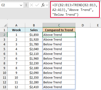
=IF(B2:B13>TREND(B2:B13,A2:A13),"Above Trend","Below Trend")
How this formula works:
- TREND(B2:B13,A2:A13) calculates the trend value for all twelve weeks at once, the same way as in Example 1.
- B2:B13>TREND(…) compares each week’s actual sales with its own trend value and gives TRUE or FALSE.
- The IF function turns each TRUE into “Above Trend” and each FALSE into “Below Trend”.
Look at week 4 and week 9. Week 4 sold $2,040 and is marked Above Trend, while week 9 sold more ($2,090) but is marked Below Trend.
That’s because sales are growing, so the trend value rises every week (from about $1,977 in week 4 to $2,223 in week 9). Comparing each week with its own trend value is fairer than comparing raw sales across weeks.
Example 4: Estimate Delivery Time From Distance
TREND isn’t only for dates and week numbers. The x-values can be any number that the y-values depend on.
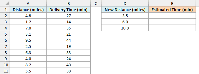
Below is a log of food deliveries with the distance and how long each one took, and I want to estimate the delivery time for three new distances in column E.
Here is the formula:
=TREND(B2:B11,A2:A11,D2:D4)
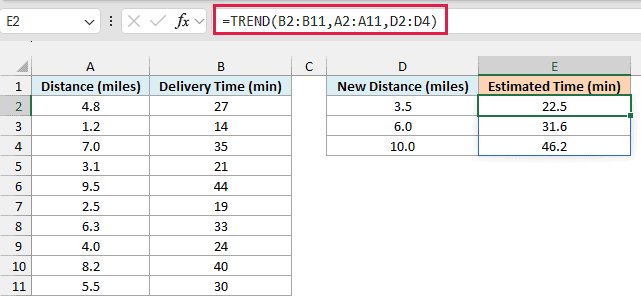
Here, A2:A11 has the distances (known_x’s) and B2:B11 has the delivery times (known_y’s). TREND works out how the time changes with distance, then estimates 22.5, 31.6, and 46.2 minutes for 3.5, 6, and 10 miles.
The log doesn’t need to be sorted by distance. TREND pairs each distance with the time in the same row, so the order of the rows doesn’t change the result.
The longest delivery in the log is 9.5 miles, so the 10-mile estimate extends the line a little past your data. Keep that in mind when you estimate values far outside the range you have.
Example 5: Predict a Value Using Two Variables
Let’s step it up with two x-variables.
Below is a list of used cars with their age, mileage, and price, and I want to estimate the price of three other cars in column G.
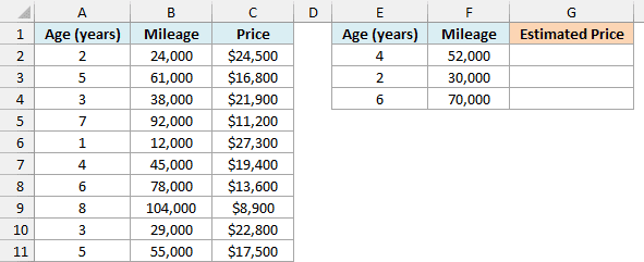
Here is the formula:
=TREND(C2:C11,A2:B11,E2:F4)
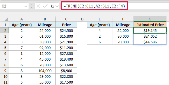
How this formula works:
- C2:C11 is known_y’s, the prices you already know.
- A2:B11 is known_x’s. Since it has two columns, TREND treats age and mileage as two separate variables.
- E2:F4 is new_x’s, the age and mileage of the three cars you want prices for.
TREND finds the combination of age and mileage that best explains the prices. It estimates $19,145 for the 4-year-old car with 52,000 miles, $24,052 for the 2-year-old car, and $14,586 for the 6-year-old car.
Important: new_x’s needs the same number of columns as known_x’s, in the same order. If you give it only the age column here (E2:E4), TREND returns the #REF! error.
Example 6: Force the Trend Line Through Zero
Now let’s look at the const argument.
Below is a log of fill-ups from a road trip with the miles driven and gallons used, and I want to estimate the gallons needed for three planned trips in columns E and F.
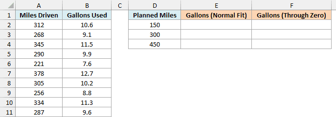
Here is the formula for the normal fit:
=TREND(B2:B11,A2:A11,D2:D4)
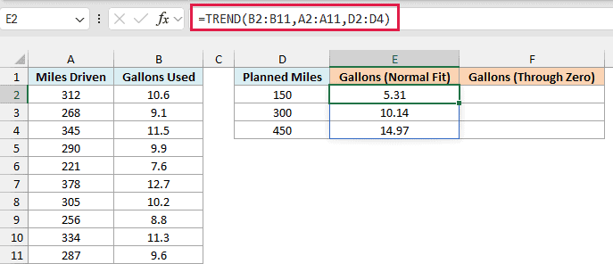
This is the normal line, and it estimates 5.31, 10.14, and 14.97 gallons for trips of 150, 300, and 450 miles.
But this line has a small problem. For a 0-mile trip it says you’d use about 0.49 gallons, which makes no sense, because driving zero miles uses zero fuel.
Here is the formula that forces the line through zero:
=TREND(B2:B11,A2:A11,D2:D4,FALSE)
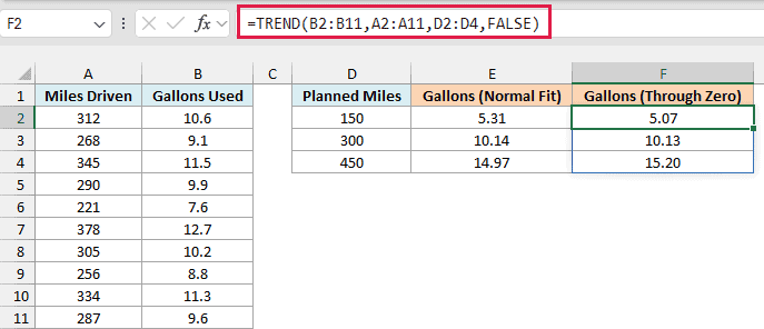
Setting const to FALSE makes the line start at zero, so 0 miles means 0 gallons. The estimates change to 5.07, 10.13, and 15.20 gallons.
Use FALSE only when a zero x-value really should give a zero y-value, like miles and fuel. For most data, leave const out and let Excel calculate the line normally.
Example 7: Fit a Curved Trend With TREND
So far, every example has used a straight line. But some data curves.
Below is a table of car stopping distances at different speeds, and I want to estimate the stopping distance at three other speeds in columns E and F.
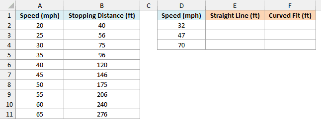
Here is the straight-line formula first:
=TREND(B2:B11,A2:A11,D2:D4)
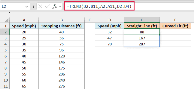
The straight line estimates 88, 167, and 287 feet. But stopping distance grows faster and faster as speed goes up, so a straight line can’t follow it, especially at 70 mph, which is past the fastest speed in the table.
Here is the formula that fits a curve instead:
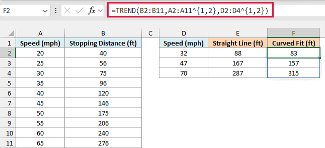
=TREND(B2:B11,A2:A11^{1,2},D2:D4^{1,2})
How this formula works:
- A2:A11^{1,2} raises each speed to the power 1 and 2. That gives TREND two columns to work with, the speed and the speed squared.
- D2:D4^{1,2} does the same for the new speeds, so new_x’s has the same two columns.
- With speed squared as a second variable (like age and mileage in Example 5), TREND fits a curve instead of a straight line.
At 70 mph, the curve estimates 315 feet while the straight line says 287 feet. That’s a 28-foot gap, and it keeps growing at higher speeds.
So these are seven practical ways to use the TREND function in Excel. I hope you found this tutorial useful.
If you only need to see the trend, adding a trendline to a chart is a quick visual option. And when you want the slope and intercept of the line, rather than the values on it, the LINEST function returns them.
Other Excel Articles You May Also Like:
