
The MAP function is a Lambda helper function that takes an array as input, applies a specified LAMBDA function to each element individually, and returns the resulting array.
Think of it as a way to process data cell-by-cell rather than all at once.
When you use a standard dynamic array calculation like =A1:A10 * B1:B10, Excel grabs the whole array at once and performs the math in a batch.
MAP, however, works differently.
It picks up one item at a time, enters a private room (the LAMBDA), performs a calculation just for that item, returns the result, and then goes back for the next one.
MAP, however, effectively says: Pause. Do not look at the whole array. Pick up one item from Array 1 and one item from Array 2, enter a private room (the LAMBDA), perform a calculation just for those items, return the result, and then go back for the next row.
This makes MAP incredibly useful when you need to apply logic that doesn’t work well with arrays, like AND, OR, or IFS functions.
Availability: Excel with Microsoft 365 and Excel on the Web
In this article, I will cover everything you need to know about the MAP function in Excel with some practical examples.
MAP Function Syntax
=MAP(array1,[array2],…,lambda)
where:
- array1 – The first array that will be processed (required).
- array2 [optional] – One or more additional arrays that the LAMBDA function needs to perform its calculation.
- lambda – A LAMBDA function that defines what transformation needs to be applied to each element (required).
The number of parameters in your LAMBDA must match the number of arrays you pass to MAP. If you have two arrays, your LAMBDA needs two parameters. If you have three arrays, your LAMBDA needs three parameters.
When to Use the MAP Function
Use this function when you need to:
- Apply cell-by-cell logic that standard array formulas can’t handle
- Use AND, OR, or IFS functions that normally don’t work correctly with arrays
- Transform each element independently while preserving the original array shape
- Combine multiple arrays element-by-element with custom logic
- Run calculations where each cell needs to be evaluated in isolation
Let me now take you through a couple of examples that will make it very clear when and how to use the MAP function in Excel.
Example 1 – Checking One Cell at a Time
Let’s start with a simple example.
I have the following dataset of 5 rows and 3 columns, and I only want to get the numbers from this dataset.
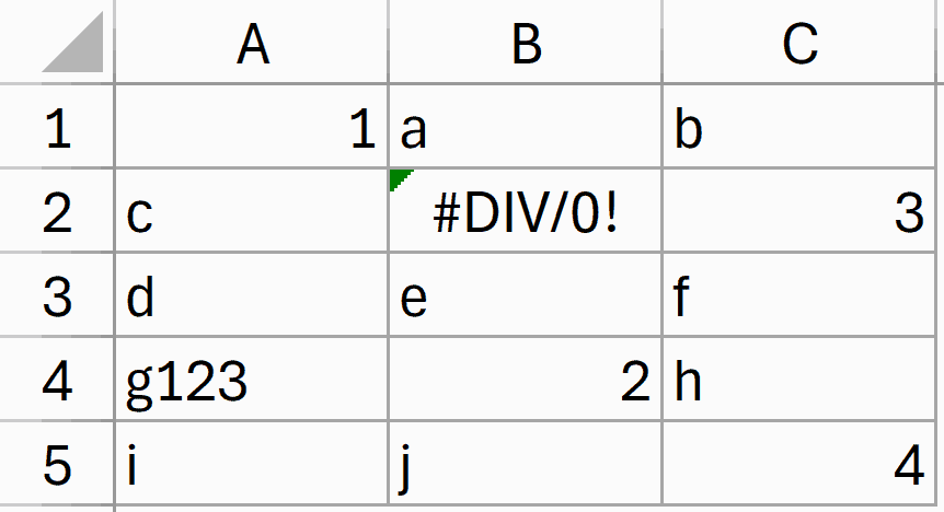
Here is a formula that will check each cell in this range, analyze it, and return the value if it’s a number; else, return a blank.
=MAP(A1:C5,LAMBDA(a,IF(ISNUMBER(a),a,"")))
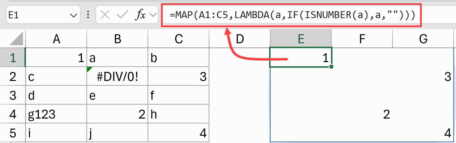
In the above formula, MAP goes through each cell in the range A1:C5 one at a time.
For each cell, it passes the value to the LAMBDA as variable a.
The LAMBDA then checks if a is a number using ISNUMBER. If it is a number, it returns that number. If not, it returns an empty string.
I have used this as the first example because I wanted to show you how the MAP function works.
You can also do the same thing using the formula below, which is shorter and cleaner (thanks to dynamic arrays).
=IF(ISNUMBER(A1:C5),A1:C5,"")
But now that you have an understanding of how the MAP function actually works by picking up each element one at a time and then applying a LAMBDA on it, let’s look at some examples where the MAP function really becomes indispensable.
Example 2: Pass/Fail Based on Multiple Conditions
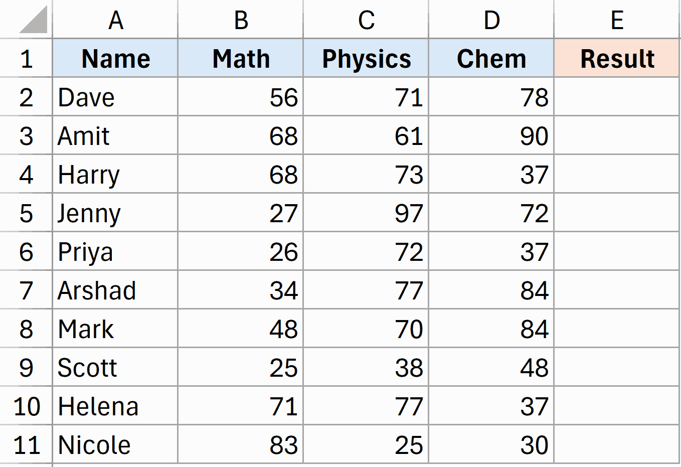
I have a dataset with student names and their scores in three subjects: Math, Physics, and Chemistry.
I want to mark students as “Pass” only if they score above 40 in Math, above 40 in Physics, AND above 50 in Chemistry.
Here is the formula:
=MAP(B2:B11, C2:C11, D2:D11, LAMBDA(a, b, c, IF(AND(a>40, b>40, c>50), "Pass", "Fail")))
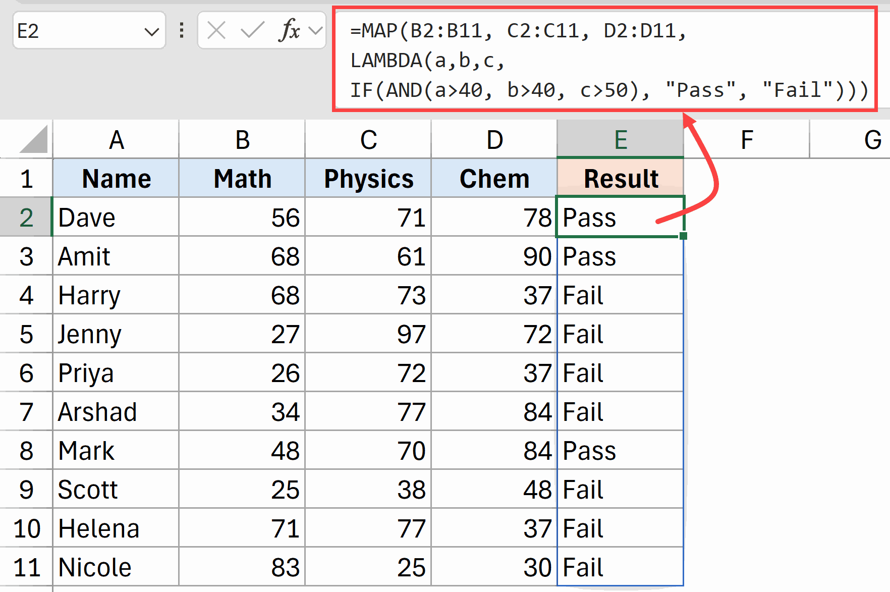
This is where MAP really shines.
Normally, if you try to use AND with arrays, it looks at ALL the values and returns a single TRUE or FALSE.
That’s not what we want.
By using MAP with three arrays, we pass one score from each subject at a time to the LAMBDA. The parameters a, b, and c hold the Math, Physics, and Chemistry scores for one student. AND then evaluates just those three values, giving us the correct row-by-row result.
Alternative approach: You can also achieve this using multiplication instead of AND:
=IF((B2:B11>40)*(C2:C11>40)*(D2:D11>50), "Pass", "Fail")
The multiplication trick works because TRUE * TRUE * TRUE = 1 and anything with FALSE becomes 0.
However, the MAP version is more readable and self-documenting, especially when you have complex conditions or when other team members need to understand the formula.
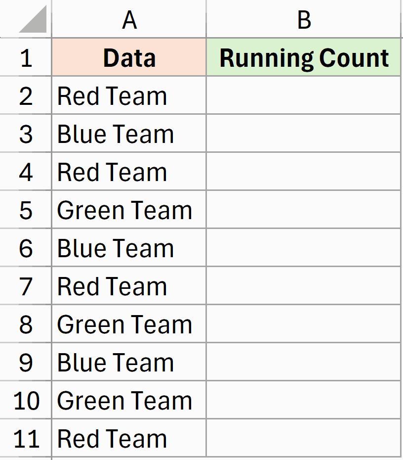
Example 3: Running Count by Category
Here’s a dataset with team names, and I want to create a running count that shows how many times each team has appeared up to that point.
Here is the formula:
=MAP(A2:A11, LAMBDA(m, COUNTIF(A2:m, m)))
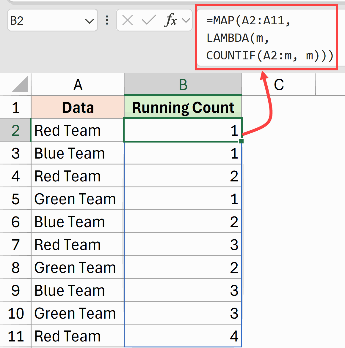
This formula is quite clever.
For each cell value m in the range, it counts how many times that value appears from A2 up to and including the current cell.
The range A2:m expands as MAP moves down the list.
So when MAP reaches the third “Red Team” entry, COUNTIF counts from A2 to that cell and finds 3 occurrences of “Red Team”. This creates a running count per category without needing helper columns.
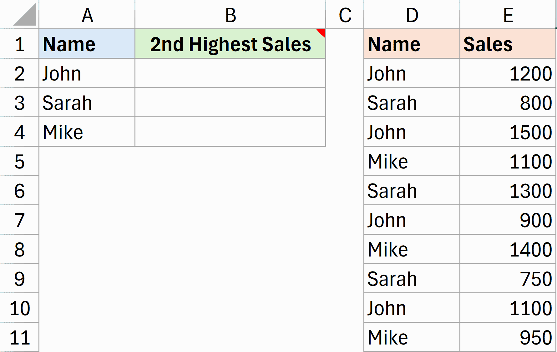
Example 4: Get 2nd Highest Sales per Person
I have a list of unique names in A2:A4, and a sales dataset in columns D and E with names and their sales figures.
I want to find the 2nd highest sales value for each person.
Here is the formula:
=MAP(A2:A4, LAMBDA(person, LARGE(FILTER(E2:E11, D2:D11=person), 2)))
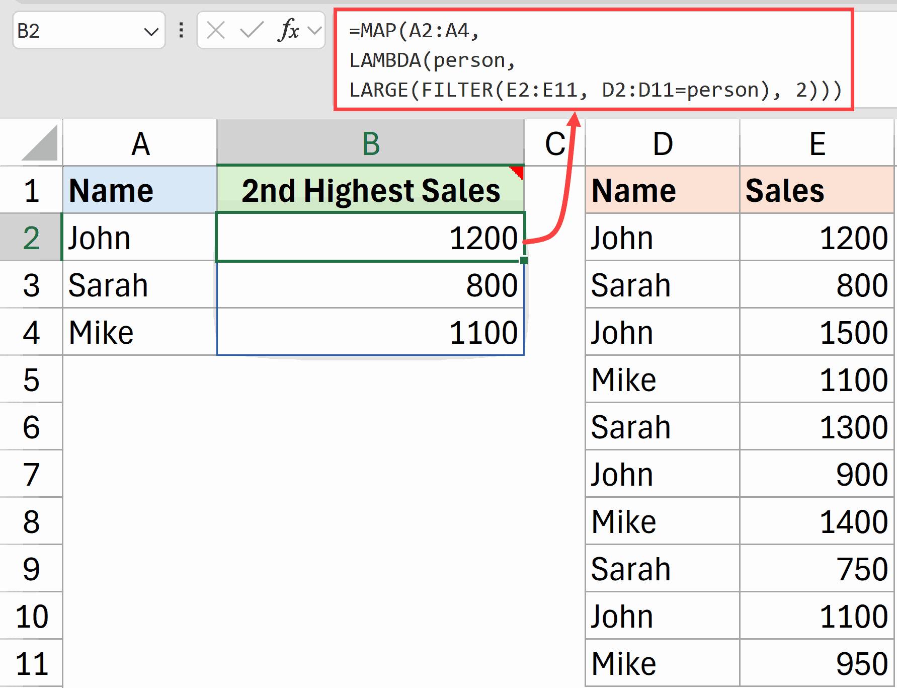
This is a more advanced example that shows the power of nesting functions inside MAP.
For each person in the list, the LAMBDA:
- Filters the sales data to get only that person’s sales
- Uses LARGE to find the 2nd highest value from the filtered results
Without MAP, you’d need to write separate formulas for each person or use complex array formulas. MAP lets you do it all in one formula that automatically processes each name.
This pattern is incredibly useful whenever you need to calculate something per category, like the highest value per region, average per department, or count per product type.
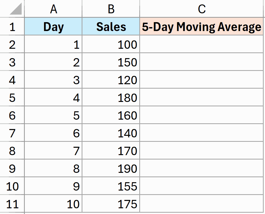
Example 5: Calculate 5-Day Moving Average
Here is an example wherethe MAP function can be very useful.
I have daily sales data and want to calculate a 5-day moving average. The average should only appear from day 5 onwards (since we need 5 days of data).
Here is the formula:
=MAP(B2:B11, LAMBDA(x, IF(ROW(x)-ROW(B$2)+1<5, "", AVERAGE(OFFSET(x, -4, 0, 5, 1)))))
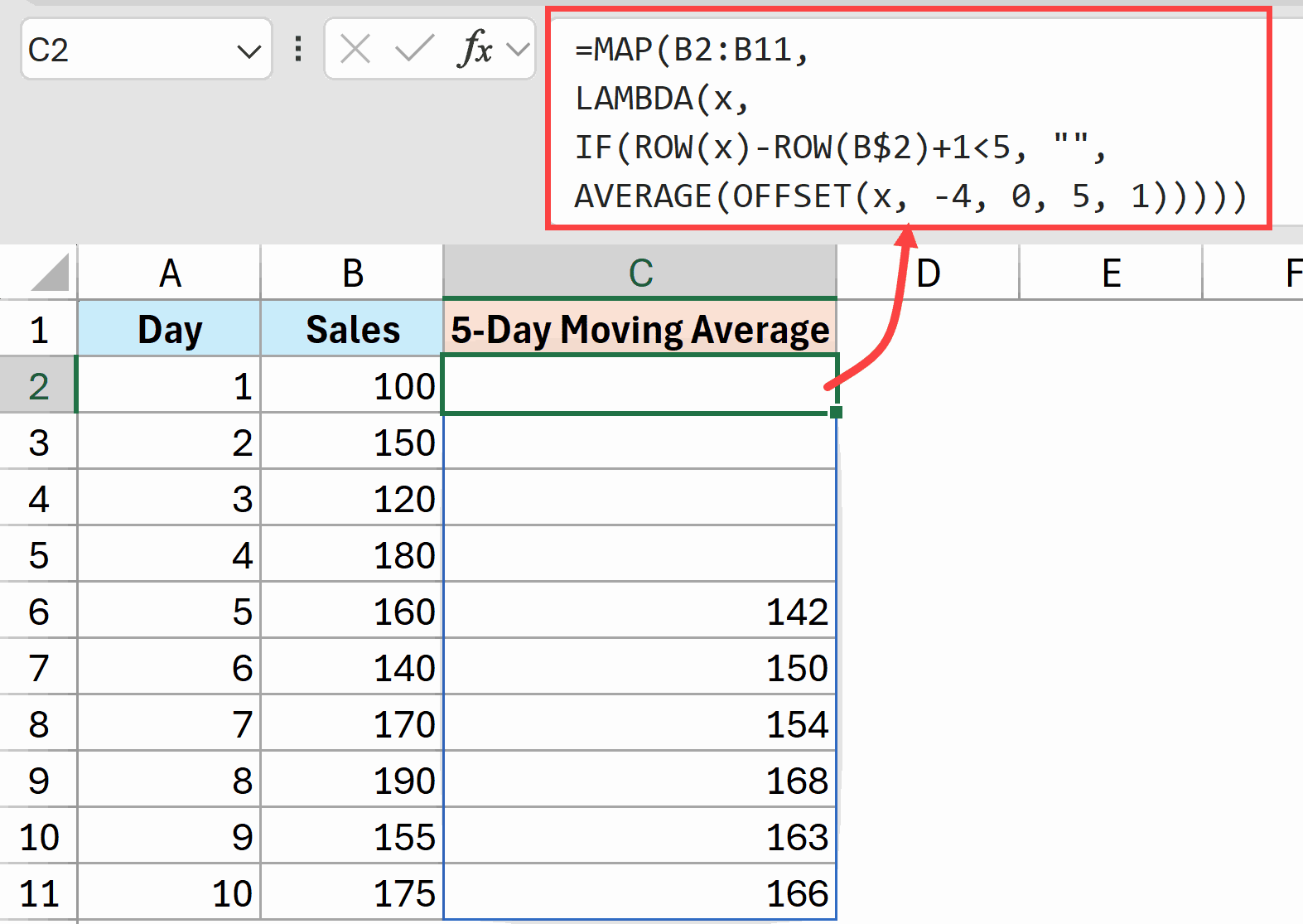
This formula calculates a moving average using MAP with OFFSET. For each sales value, the LAMBDA first checks if we’re at row 5 or beyond (we need at least 5 data points).
If not, it returns empty. If yes, it uses OFFSET to grab the 5 cells ending at the current cell and calculates their average.
The expression ROW(x)-ROW(B$2)+1 figures out which row number we’re on relative to the start of our data. OFFSET then creates a range of 5 cells going up from the current position.
Without MAP, you’d need a helper column with formulas copied down each row. MAP gives you a clean, single-formula solution.
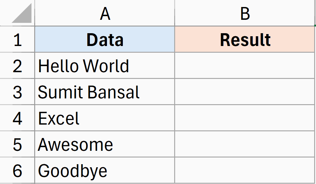
Example 6: Reverse Text Strings
And finally, here’s an example that shows what’s possible with MAP, even if it’s not something you’d use every day.
I have a list of text values and want to reverse each one (so “Hello World” becomes “dlroW olleH”).
Here is the formula:
=MAP(A2:A6, LAMBDA(txt, TEXTJOIN("", TRUE, MID(txt, SEQUENCE(LEN(txt), 1, LEN(txt), -1), 1))))
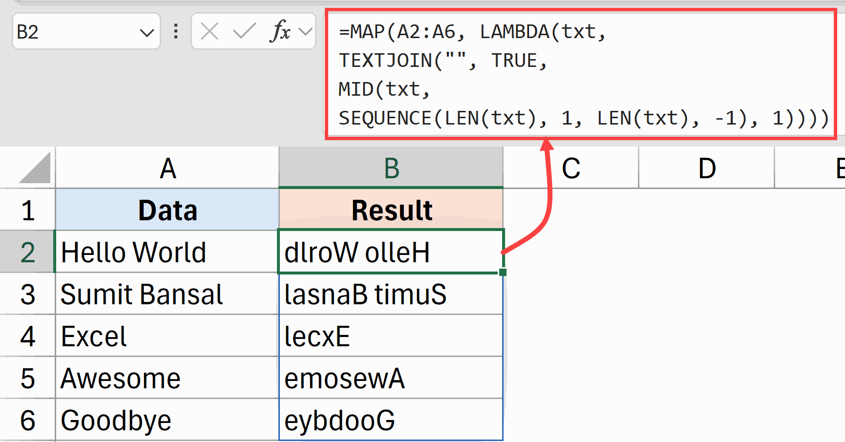
While reversing text isn’t a common task, this example demonstrates that MAP can work with character-level processing. The formula:
- Uses SEQUENCE to create numbers from the length of the text down to 1
- Uses MID to extract each character in reverse order
- Uses TEXTJOIN to combine all the characters back together
The key insight is that MAP lets us apply this complex character manipulation to each cell in a range, all in one formula.
Without MAP, the TEXTJOIN/MID/SEQUENCE combination would only work on a single cell at a time.
Tips & Common Mistakes
- Match LAMBDA parameters to arrays: If you pass 3 arrays to MAP, your LAMBDA must have 3 parameters. Mismatching causes a #VALUE! error.
- LAMBDA must return a single value: MAP expects each calculation to return one value per cell. If your LAMBDA returns an array (like TEXTSPLIT), you’ll get a #CALC! “Nested Array” error. Wrap array-returning functions in an aggregator like TEXTJOIN or COUNTA.
- Don’t use MAP for simple math: For basic operations like multiplication or addition, native array formulas (=A1:A10 * 2) are much faster than MAP. Reserve MAP for logic that truly needs cell-by-cell processing.
- MAP vs BYROW: Use MAP when you need to work with individual cells. Use BYROW when you need to work with entire rows (like summing across columns).
- Preserves array shape: MAP always returns an array with the same dimensions as the input. A 5×3 input produces a 5×3 output.
- Availability: MAP only works in Excel 365 and Excel for the Web. Users on Excel 2019 or earlier will see a #NAME? error.
The MAP function opens up possibilities that were previously only achievable with VBA or complex helper columns.
Once you understand its cell-by-cell approach, you’ll find many situations where it simplifies otherwise complicated formulas.
Start with the simpler examples and work your way up to combining MAP with other functions like FILTER, REDUCE, and LARGE.
Other Excel articles you may also like:


