

The RECEIVED function in Excel calculates the amount you’ll get at maturity from a discounted security, using the amount invested, an annual discount rate, and the purchase and maturity dates.
That makes it useful when money is paid upfront and returned as one amount at the end. The result includes your original investment, so you’ll need to subtract that investment if you want just the gain.
In this tutorial, I’ll show you four examples, including a single investment, several investment amounts, and a comparison of day-count conventions. RECEIVED needs a small adjustment to handle a range of cells, which I’ll explain in the second example.
Follow along with the example file
RECEIVED Function Examples.xlsx
RECEIVED Function Syntax
Here is the syntax of the RECEIVED function:
=RECEIVED(settlement, maturity, investment, discount, [basis])
- settlement is the date you buy the security. Supply a reference to a cell containing a real Excel date, or a date created with the DATE function.
- maturity is the date the security pays out. It must be later than the settlement date.
- investment is the amount paid upfront. Enter it as a positive number.
- discount is the positive annual discount rate quoted for the security. Enter 4.8% as
4.8%or0.048. - basis is optional and tells Excel how to count the days between the two dates. If you leave it out, Excel uses 0, the US (NASD) 30/360 convention.
The discount rate is applied to the amount paid at maturity, rather than to the amount you invest. This is why you can’t replace it with an ordinary savings-account interest rate and expect the same result.
Here are the five basis options:
| Basis | Day-count Convention |
|---|---|
| 0 or omitted | US (NASD) 30/360 |
| 1 | Actual/Actual |
| 2 | Actual/360 |
| 3 | Actual/365 |
| 4 | European 30/360 |
The basis controls the fraction of a year used in the calculation. For example, basis 2 counts the actual days between the dates and divides that number by 360.
Excel drops fractional parts from the settlement, maturity, and basis arguments. So a time attached to a date doesn’t add a partial day, and basis 2.9 is treated as 2.
RECEIVED is available in Excel 365, 2024, 2021, 2019, and 2016, including the corresponding Mac versions. The spilling examples below use dynamic-array Excel, such as Microsoft 365, 2024, or 2021.
When to Use the RECEIVED Function
Use this function when you need to:
- Calculate the maturity amount of a discounted security from its purchase amount and quoted discount rate.
- Work out maturity proceeds for several investment amounts under the same terms.
- Check how a day-count convention affects the calculation.
- Find the monetary gain before fees and taxes by subtracting the original investment.
Let me show you how these calculations work in the example file.
Example 1: Calculate One Maturity Amount
Let’s start with one investment so you can see how the arguments fit together.
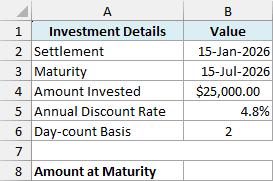
Below are the terms for a $25,000 investment settled on January 15, 2026, and maturing on July 15, 2026, and I want the amount received at maturity in cell B8.
On the Single Investment sheet, enter this formula in B8:
=RECEIVED(B2,B3,B4,B5,B6)
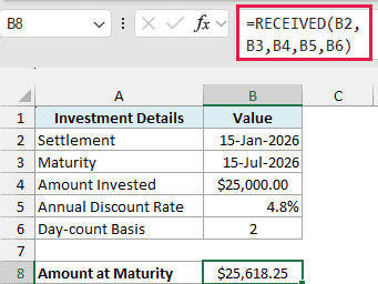
The result is $25,618.25, displayed to two decimal places. This is the total paid at maturity, including the $25,000 invested.
In the above formula, B2 and B3 supply the dates, B4 supplies the investment, and B5 supplies the 4.8% annual discount rate. The 2 in B6 tells Excel to use Actual/360.
There are 181 days between these dates. RECEIVED divides $25,000 by 1 - 0.048 * 181 / 360, which gives $25,618.2538598 before display rounding.
That division is the part to notice. Adding 4.8% interest to $25,000 for the same fraction of a year would use a different calculation because the quoted discount is based on the maturity amount.
Important: Both the investment and discount must be greater than zero, and maturity must be later than settlement. Otherwise, RECEIVED returns #NUM!, so a zero-rate investment also needs a different calculation.
If a date is stored as text, changing its display format won’t turn it into a real date. An unrecognized date can cause #VALUE!; you can convert text to dates before using the function.
If you’re entering dates directly in a formula, the DATE function avoids ambiguous text such as “04/05/2026”, which different regional settings can read as April 5 or May 4.
Example 2: Calculate Several Investment Amounts
Now let’s use the same terms for several amounts invested.
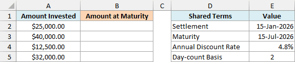
Below are four possible investment amounts with shared dates and a 4.8% annual discount rate, and I want their maturity proceeds in column B.
On the Several Investments sheet, enter this formula in B2:
=RECEIVED(E2,E3,+A2:A5,E4,E5)
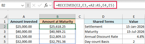
The formula returns four amounts automatically: $25,618.25, $40,989.21, $12,809.13, and $32,791.36. They correspond to the investments in the same row.
E2 and E3 provide the dates, while E4 and E5 provide the discount rate and basis. Because those terms are shared, only the investment amount changes for each result.
The plus sign before A2:A5 converts the range into an array of values that RECEIVED can calculate with. It doesn’t add anything to the investment amounts.
Important: Passing A2:A5 directly to RECEIVED returns #VALUE! in this example. Keep the plus sign before the range, and keep B3:B5 empty so the results have room to spill.
If the output cells already contain something, Excel shows #SPILL! instead of filling them. Clear those cells and leave the formula only in B2.
If you are using Excel 2019 or earlier, enter the below formula in B2 and copy it down to B5:
=RECEIVED($E$2,$E$3,A2,$E$4,$E$5)
The dollar signs keep the shared terms fixed while A2 changes to the investment on each row. This version handles one investment at a time, so it doesn’t need the plus sign.
Example 3: Compare Day-count Conventions
The basis argument can change the answer even when every other input stays the same.
Below are all five day-count conventions for an $18,500 investment from February 28 to August 31, 2026, and I want the maturity amount for each convention in column C.
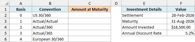
On the Day-count Comparison sheet, enter this formula in C2:
=RECEIVED(F2,F3,F4,F5,+A2:A6)
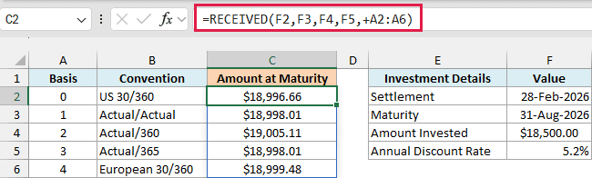
The results range from $18,996.66 for US 30/360 to $19,005.11 for Actual/360. The investment, dates, and 5.2% annual discount rate stay fixed; the basis code changes for each row.
The plus sign serves the same purpose as in Example 2. Here it converts the five basis codes into values so RECEIVED can return one amount per convention.
Actual/360 uses the 184 actual days between the dates and divides by 360. Actual/365 divides those same 184 days by 365, giving $18,998.01.
Actual/Actual also gives $18,998.01 in this example because the dates fall within the same non-leap year. Don’t assume it always matches Actual/365 when you change the dates.
The two 30/360 conventions apply different month-end rules. With these February and August dates, US 30/360 gives $18,996.66, while European 30/360 gives $18,999.48.
Important: Use the basis specified for the security, rather than whichever produces the largest amount. Leaving basis out selects US 30/360, and a whole-number code outside 0 through 4 returns #NUM!.
If you are using Excel 2019 or earlier, enter the below formula in C2 and copy it down to C6:
=RECEIVED($F$2,$F$3,$F$4,$F$5,A2)
Example 4: Find the Gain at Maturity
For the last example, let’s separate the gain from the original investment.
Below are the terms of a $48,000 investment at a 4.6% annual discount rate, and I want the gain before fees and tax in cell B8.
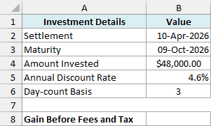
On the Gain at Maturity sheet, enter this formula in B8:
=RECEIVED(B2,B3,B4,B5,B6)-B4
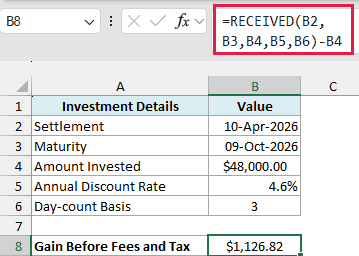
The result is $1,126.82. RECEIVED calculates $49,126.82 at maturity, and subtracting B4 removes the $48,000 originally invested.
The dates run from April 10 to October 9, 2026, a period of 182 days. Basis 3 uses Actual/365, so the calculation uses 182/365 of a year.
This result is a dollar gain, not a return percentage or an annualized rate. Fees and taxes aren’t inputs to RECEIVED, so the result doesn’t deduct them.
In this tutorial, I showed you how to calculate maturity proceeds, handle several investments, and separate the gain from the total. Make sure the discount rate and day-count basis match the security’s terms before using your own figures.
I hope you found this article helpful.
Other Excel Articles You May Also Like:
