

The PRICEMAT function in Excel calculates the price per $100 face value of a security that pays all its interest at maturity. You give it the security’s dates, interest rate, and required yield, and it returns a price you can compare with a quote.
That price excludes interest already earned before the buyer takes ownership. I’ll show you how to calculate the price, choose the day-count basis, and work out the cash needed for a purchase.
PRICEMAT doesn’t handle a range of yields directly in the tested Excel version. The last example uses the MAP function to calculate several prices with one formula.
Follow along with the example file
PRICEMAT Function Examples.xlsx
PRICEMAT Function Syntax
Here is the syntax of the PRICEMAT function:
=PRICEMAT(settlement, maturity, issue, rate, yld, [basis])
- settlement is the date the buyer takes ownership of the security. Enter a real Excel date or a reference to a date cell.
- maturity is the date the security repays its principal and interest. This must be later than settlement.
- issue is the date the security was originally issued, when interest starts accumulating. This is separate from the date you buy it.
- rate is the annual interest rate set when the security was issued. Enter 5% as
5%or0.05. - yld is the annual yield required by the buyer. It can differ from the security’s interest rate, so enter the two rates separately.
- basis is an optional number that tells Excel how to count days. If you leave it out, Excel uses 0, or US (NASD) 30/360.
The basis choices are:
| Basis | Day-count method |
|---|---|
| 0 or omitted | US (NASD) 30/360 |
| 1 | Actual/actual |
| 2 | Actual/360 |
| 3 | Actual/365 |
| 4 | European 30/360 |
The 30/360 methods use adjusted 30-day months and a 360-day year. The actual methods count calendar days, then use the year length specified by the basis; US and European 30/360 differ in how they handle some month-end dates.
Excel ignores fractional parts of the date and basis arguments. Use whole-number basis codes so the calculation doesn’t silently use a different convention than you intended.
PRICEMAT works in Excel for Microsoft 365, Excel 2024, 2021, 2019, and 2016, including supported Mac editions. The MAP example below requires Microsoft 365 or Excel 2024.
When to Use the PRICEMAT Function
Use this function when you need to:
- Calculate a quote for a security that pays its interest at maturity.
- Compare prices under different day-count conventions.
- Convert a price per $100 into an amount for your investment.
- See how changing the required yield changes the price.
Let’s work through these using the four sheets in the example workbook.
Example 1: Calculate a Security’s Clean Price
Let’s start with one security and one required yield.
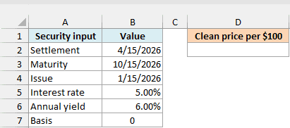
Below are the terms of a note that pays interest at maturity, and I want its price per $100 in cell D2 on the Example 1 sheet.
Enter this formula in D2:
=PRICEMAT(B2,B3,B4,B5,B6,B7)
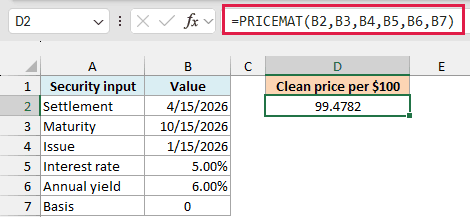
The result is 99.4782, displayed to four decimal places. This means a clean price of about $99.48 for each $100 of face value, where face value is the principal repaid at maturity.
The note earns 5% interest from January 15 to October 15, 2026. The buyer takes ownership on April 15 and requires a 6% annual yield, so the formula calculates the price for that purchase date.
A clean price excludes interest accumulated from issue to settlement. The buyer normally pays that accrued interest as well, which we’ll calculate in Example 3.
The dates in the workbook are real Excel dates. If your formula returns #VALUE!, check for dates stored as text.
The DATE function can build a date from separate year, month, and day values. This avoids relying on how Excel interprets a text date.
Negative interest rates or yields return #NUM!. You’ll also get #NUM! if the settlement date is the maturity date or later, so check those inputs before changing the formula.
Example 2: Compare Day-Count Bases
Keep the security’s terms the same while changing how Excel counts the days.
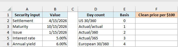
Below are the five basis choices on the Example 2 sheet, and I want the corresponding prices in column F.
Enter this formula in F2, then copy it down to F6:
=PRICEMAT($B$2,$B$3,$B$4,$B$5,$B$6,E2)
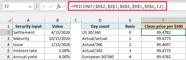
The dollar signs keep the dates and rates fixed as you copy the formula. The reference to E2 changes to E3, E4, and so on, so each row uses its own basis code.
US 30/360 gives 99.4782, while Actual/360 gives 99.4697. The prices are close, but they’re not interchangeable when you need to match a quote based on the security’s terms.
Actual/actual and Actual/365 both give 99.4773 here because all the dates fall within the same non-leap year. Their matching results in this example don’t mean the two conventions always match.
Choose the basis specified for the security. A basis outside 0 through 4 returns #NUM!; leaving it out silently selects US 30/360, which may not be the convention you need.
Important: Keep PRICEMAT’s inputs scalar here. Direct range input returned #VALUE! in native Excel testing, so this example copies the formula down; Example 4 uses MAP to pass one scenario value at a time.
Example 3: Calculate the Cash Settlement Amount
The quote is per $100, but your purchase may have a much larger face value.
Below are the same note’s terms with a $25,000 face value on the Example 3 sheet, and I want the purchase amounts in column E.
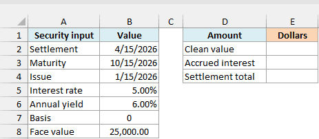
First, enter this formula in E2 to calculate the clean value of the position:
=PRICEMAT(B2,B3,B4,B5,B6,B7)/100*B8
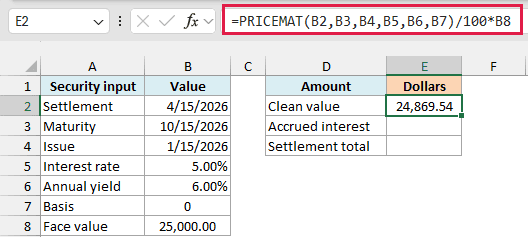
The result is $24,869.54. Dividing the quote by 100 converts it to a proportion of face value, and multiplying by B8 scales it to the $25,000 position.
Next, calculate the interest earned from issue to settlement in E3:
=ACCRINTM(B4,B2,B5,B8,B7)
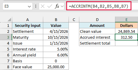
The ACCRINTM function gives $312.50. Here we use the purchase settlement date as the accrual endpoint, so it calculates only the interest earned before this buyer takes ownership.
On the selected 30/360 basis, January 15 to April 15 is 90 days. The accrued amount is therefore $25,000 multiplied by 5%, multiplied by 90/360.
Finally, enter this formula in E4 to add the two amounts:
=SUM(E2:E3)
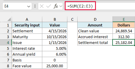
The settlement total is $25,182.04, before fees. This is the cash amount including accrued interest, often called the dirty value of the position.
The clean quote is below 100, yet the settlement total is above the $25,000 face value because it includes accrued interest. Keep the full formula precision for these calculations and format the final dollar amounts to two decimal places.
Example 4: Compare Several Required Yields
Now let’s see how the price changes when the buyer requires a different return.
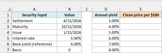
Below are six possible yields for the same note on the Example 4 sheet, and I want all six prices in column E.
In Excel for Microsoft 365 or Excel 2024, enter this formula in E2:
=MAP(D2:D7,LAMBDA(y,PRICEMAT(B2,B3,B4,B5,y,B7)))
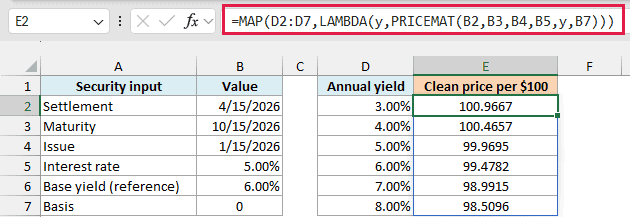
The MAP function takes each yield from D2:D7 and passes it to the calculation as y. PRICEMAT receives one yield at a time, and MAP returns the six prices into E2:E7.
The reference yield in B6 shows the original 6% assumption for comparison. This formula uses the scenario yields in column D instead of B6.
At a 3% required yield, the clean price is 100.9667. At 8%, it falls to 98.5096, because a buyer requiring a higher return pays less for the same future payment.
Even when the yield equals the note’s 5% interest rate, the price is 99.9695, not exactly 100. PRICEMAT discounts the maturity payment and subtracts the interest accrued before settlement; equal annual rates alone don’t guarantee a clean price of 100.
If Excel returns #SPILL!, something is blocking the output cells below E2. Clear those cells so the six results can appear.
If you’re using Excel 2021, 2019, or 2016 without MAP, enter the formula below in E2 and copy it down to E7:
=PRICEMAT($B$2,$B$3,$B$4,$B$5,D2,$B$7)
These examples show how to go from a PRICEMAT quote to a cash settlement amount and compare yield assumptions. For a bond that pays interest periodically during its life, use the PRICE function instead.
Other Excel Articles You May Also Like:
