

The ODDLPRICE function in Excel gives you the price of a bond whose last coupon period is odd, meaning it’s shorter or longer than the bond’s normal payment period. Like the other bond price functions, it returns the price per $100 of face value.
This comes up when a bond’s maturity date doesn’t line up with its regular coupon schedule. The regular PRICE function assumes every period is the same length, so ODDLPRICE is the one to use for that irregular final stretch.
Below, I’ll price bonds with short and long last periods, price a whole list with one formula, track the price as maturity gets closer, and work out the full amount you’d pay.
Follow along with the example file
ODDLPRICE Function Examples.xlsx
ODDLPRICE Function Syntax
Here is the syntax of the ODDLPRICE function:
=ODDLPRICE(settlement,maturity,last_interest,rate,yld,redemption,frequency,[basis])
- settlement – the date you buy the bond. It has to fall after the last coupon date.
- maturity – the date the bond matures and pays back its face value.
- last_interest – the bond’s last regular coupon date before maturity.
- rate – the bond’s annual coupon rate, such as 4.25%.
- yld – the annual yield you want to earn on the bond, such as 5.10%.
- redemption – the amount the bond pays back at maturity per $100 of face value. For most bonds, this is 100.
- frequency – the number of coupon payments per year. Use 1 for annual, 2 for semiannual, and 4 for quarterly.
- [basis] – optional. The day count method: 0 (US 30/360), 1 (actual/actual), 2 (actual/360), 3 (actual/365), or 4 (European 30/360). If you leave it out, Excel uses 0.
The stretch from last_interest to maturity is the odd last period. If it’s shorter than one normal coupon period, it’s a short last period, and if it’s longer, it’s a long one.
You don’t tell ODDLPRICE which kind it is. It works that out from the dates and the frequency.
The three dates have to be in this order: last_interest, then settlement, then maturity. If they aren’t (for example, the settlement date is on or before the last coupon date), ODDLPRICE returns the #NUM! error.
The frequency only accepts 1, 2, or 4. Any other number, like 12 for a monthly bond, also returns #NUM!, and so does a negative coupon rate or yield.
The dates should be real dates in cells, or dates built with the DATE function. If Excel can’t read a date, ODDLPRICE returns the #VALUE! error.
The ODDLPRICE function works in Excel 365, 2024, 2021, 2019, 2016, and Excel for Mac.
When to Use the ODDLPRICE Function
Use this function when you need to:
- Price a bond whose final coupon period is shorter or longer than the rest
- Price a whole list of bonds with odd last periods in one go
- See how a bond’s price changes as its maturity date gets closer
- Work out the full price you pay, including the interest built up since the last coupon
Let me show you a few practical examples of how to use the ODDLPRICE function.
Example 1: Price a Bond With a Short Last Coupon Period
Let’s start with a simple example.
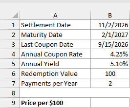
Below are the details of a bond that pays coupons twice a year and has a short last coupon period, and I want its price in cell B9.
Here is the formula:
=ODDLPRICE(B1,B2,B3,B4,B5,B6,B7)
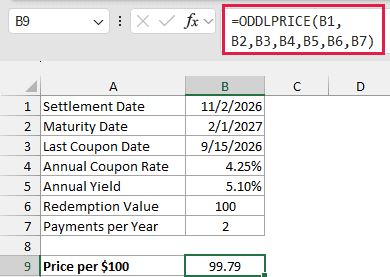
The formula returns 99.79, which is below 100. That’s because the bond’s 4.25% coupon is lower than the 5.10% yield, so the only way to earn 5.10% is to pay less than the 100 you get back.
The last coupon period here is short. The last coupon is on September 15, 2026, and the bond matures on February 1, 2027, about 4.5 months later instead of the usual 6.
If you used the PRICE function on this bond instead, you’d get 99.78. PRICE assumes the coupons run every six months counting back from maturity, so it works from an August 1, 2026 coupon date that this bond never had.
The gap is small here, but 99.79 is the right price for this bond. And since both results are per $100 of face value, the difference grows with the size of your holding.
Important: Enter the coupon rate and yield as percentages (4.25% and 5.10%) or decimals (0.0425 and 0.051). If you type 4.25 and 5.1 instead, ODDLPRICE doesn’t show an error, but it returns a wrong price (59.76 for this bond).
Example 2: Price a Bond With a Long Last Coupon Period
Now let’s look at a bond with a long last coupon period.
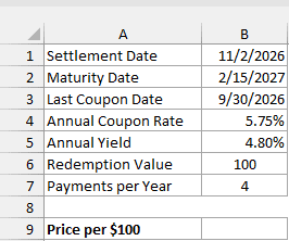
Below are the details of a bond that pays coupons four times a year, and I want its price in cell B9.
Here is the formula:
=ODDLPRICE(B1,B2,B3,B4,B5,B6,B7)
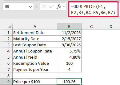
The formula returns 100.26. This time the price is above 100, because the 5.75% coupon is higher than the 4.80% yield, so the bond is worth paying a little extra for.
With quarterly payments, a normal coupon period is 3 months. The last coupon is on September 30, 2026, and maturity is February 15, 2027, about 4.5 months later, so this last period is long.
Notice that both bonds so far have a last period of about 4.5 months. That’s short for a bond that pays twice a year and long for one that pays four times a year, which is why the Payments per Year value in B7 matters.
Example 3: Price a List of Bonds With One ODDLPRICE Formula
Here’s another practical scenario where you have several bonds to price.
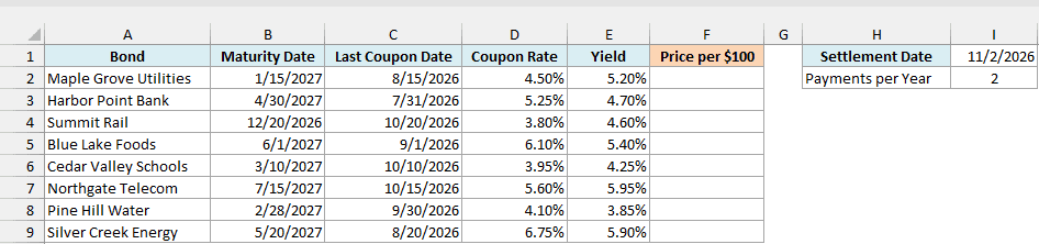
Below is a list of eight bonds with their maturity dates, last coupon dates, coupon rates, and yields, and I want the price of each bond in column F, using the settlement date in I1 and the payments per year in I2.
Here is the formula:
=ODDLPRICE(I1,+B2:B9,+C2:C9,+D2:D9,+E2:E9,100,I2)
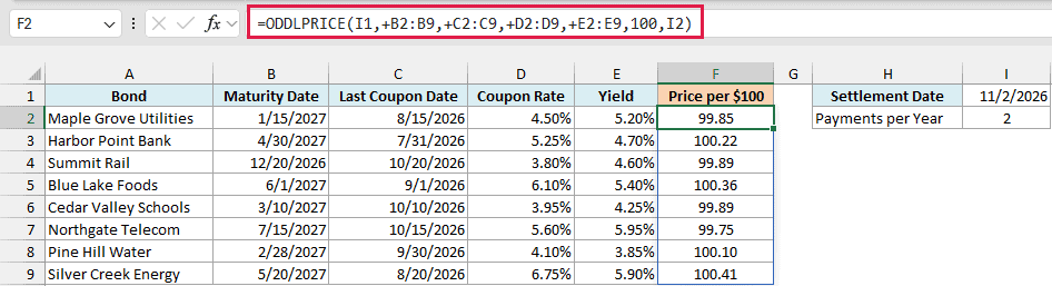
This formula spills all eight prices into F2:F9. The plus sign in front of each range is what makes that work.
ODDLPRICE doesn’t accept a cell range in these arguments. The plus sign hands it the values in the range instead, so it can return one price for each bond.
Important: If you leave out the plus sign and use a plain range like B2:B9, ODDLPRICE returns a single #VALUE! error instead of spilling. Every range in the formula needs its own plus sign.
Each bond uses its own maturity date, last coupon date, coupon rate, and yield, while the settlement date in I1 and the 2 payments per year in I2 apply to every bond.
I’ve typed the redemption value of 100 straight into the formula, since it’s the same for every bond. You could also keep it in a cell, like in the first two examples.
The list mixes both kinds of odd periods. Summit Rail’s last period is only 2 months long (short), while Harbor Point Bank’s runs 9 months (long), and the same formula prices both.
If you are using Excel 2019 or earlier, enter the below formula in cell F2 and then copy it down the range:
=ODDLPRICE($I$1,B2,C2,D2,E2,100,$I$2)
Example 4: See How the Bond Price Changes as Maturity Gets Closer
Now let’s look at something a bit more interesting.
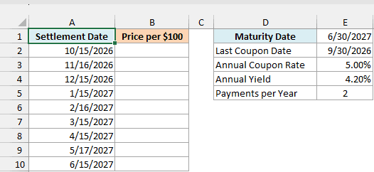
Below is a list of possible settlement dates for one bond, and I want the bond’s price on each of those dates in column B, using the bond details in column E.
Here is the formula:
=ODDLPRICE(+A2:A10,E1,E2,E3,E4,100,E5)
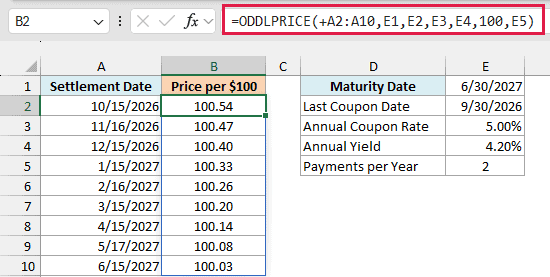
The formula spills nine prices into B2:B10, one for each settlement date. Only the settlement dates change, so A2:A10 is the only range that needs the plus sign.
The price drops from 100.54 in October 2026 to 100.03 in June 2027. This bond’s 5% coupon is above its 4.20% yield, so it starts above 100, and that extra shrinks as the bond gets closer to paying back its 100 at maturity.
This is useful when you’re deciding when to buy or sell, because you can see what the bond is worth at the same yield on different dates.
If you are using Excel 2019 or earlier, enter the below formula in cell B2 and then copy it down the range:
=ODDLPRICE(A2,$E$1,$E$2,$E$3,$E$4,100,$E$5)
Example 5: Calculate the Full Price of a Bond (Clean Price Plus Accrued Interest)
Let’s step it up with something ODDLPRICE doesn’t give you on its own.
ODDLPRICE returns the clean price, which leaves out the interest the bond has built up since its last coupon. When you buy a bond between coupon dates, you also pay the seller that accrued interest.
The clean price plus the accrued interest is the full price (also called the dirty price).
Below are the details of a bond, and I want its clean price in B8, the accrued interest in B9, and the full price in B10.
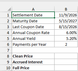
Here is the formula for the clean price:
=ODDLPRICE(B1,B2,B3,B4,B5,100,B6)
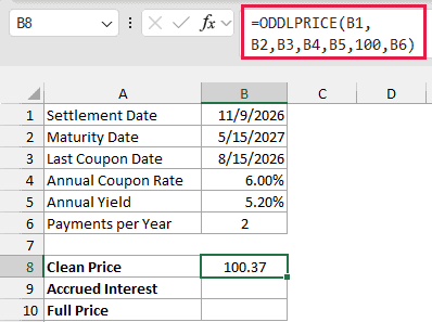
This is the regular ODDLPRICE formula, and it returns 100.37 per $100 of face value. That’s the price you’d usually see quoted.
Here is the formula for the accrued interest:
=ACCRINT(B3,B2,B1,B4,100,B6)
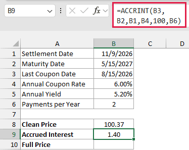
How this formula works:
- B3 (the last coupon date, August 15, 2026) goes in the issue argument of the ACCRINT function, so it counts interest starting from the last coupon payment.
- B2 (the maturity date) is the next interest payment date, because the bond’s final coupon is paid at maturity.
- B1 is the settlement date, where the counting stops.
- B4, 100, and B6 are the 6% coupon rate, the $100 of face value, and the 2 payments per year.
That gives 1.40, which is 84 days of interest at 6% a year on $100, counted the US 30/360 way.
That’s the same day count ODDLPRICE uses when you leave out its basis argument. If your bond uses a different basis, give both functions the same basis code.
And here is the formula for the full price:
=B8+B9
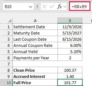
Adding the two gives a full price of 101.77 per $100 of face value. This is what you actually pay, even though the quote you’d see is 100.37.
So these are five practical ways to use the ODDLPRICE function. Give it the real last coupon date, keep the three dates in order, and add the plus sign in front of any range you feed it.
If the odd period is at the start of a bond’s life instead of the end, the ODDFPRICE function is the one built for that case.
Other Excel Articles You May Also Like:
