

Excel now has three new REGEX functions, which allow us to work with text data a lot more efficiently.
These functions are available in Excel for Microsoft 365 on Windows and Mac.
- REGEXEXTRACT
- REGEXREPLACE
- REGEXTEST
While Excel already has many text functions and functionalities to deal with text manipulation, REGEX functions can be quite helpful in some situations.
REGEX is not a new concept and has been around for more than 50 years. It’s only now that we have got it in Excel.
In this article, I will show you some practical examples of how you can use these new regex functions in Excel.
So let’s get started!
Click here to download the example file and follow along
Follow along with the example file
REGEX Functions Examples.xlsx
Regex Metacharacters (Tokens) Table with Examples
Below is a table where I have listed all the Regex meta characters along with their explanation and an example.
You’re not expected to remember all of these, but you can bookmark this page so that you can come back and refer to it whenever needed.
The usage of these tokens becomes a lot clearer when you start looking at the example covered later in this article.
| Metacharacter | Name | What it does | Examples |
|---|---|---|---|
| . | Dot | Matches any single character except newline (unless configured otherwise) | a.c matches “abc”, “a1c”, “a@c”, but not “a\nc” |
| | | Pipe | Acts as an OR operator, allowing either the expression before or after it to match | cat|dog matches “cat” or “dog” |
| * | Asterisk | Matches the preceding character or group zero or more times (greedy) | ab*c matches “ac”, “abc”, “abbc”, “abbbc”, etc. |
| ^ | Caret | Anchors the match to the beginning of the string or line | ^Hello matches “Hello World” but not “World Hello” |
| $ | Dollar | Anchors the match to the end of the string or line | World$ matches “Hello World” but not “World Hello” |
| + | Plus | Matches the preceding character or group one or more times (greedy) | ab+c matches “abc”, “abbc”, “abbbc”, but not “ac” |
| \ | Backslash | Escapes the following character, treating metacharacters as literals or giving special meaning to ordinary characters | \. matches a literal dot, \d matches any digit |
| ? | Question mark | Makes the preceding character or group optional, matching it zero or one time | colou?r matches both “color” and “colour” |
| [] | Brackets | Defines a character set, matching any single character within the brackets | [aeiou] matches any single vowel |
| {} | Braces | Specifies an exact number or range of occurrences for the preceding character or group | a{2,4} matches “aa”, “aaa”, and “aaaa” |
| () | Parentheses | Groups characters together and creates a capturing group | (ab)+ matches “ab”, “abab”, “ababab”, etc. |
| (?:) | Non-capturing group | Groups characters without creating a capturing group | (?:ab)+ same as above, but doesn’t create a capture |
| \d | Digit | Matches any digit (equivalent to [0-9]) | \d{3} matches “123”, “456”, etc. |
| \w | Word character | Matches any word character (equivalent to [a-zA-Z0-9_]) | \w+ matches “hello_world123” |
| \s | Whitespace | Matches any whitespace character (spaces, tabs, newlines) | a\sb matches “a b”, “a\tb”, “a\nb” |
| \b | Word boundary | Matches a position where a word starts or ends | \bcat\b matches “cat” in “The cat sat” but not in “category” |
| [^] | Negated set | Matches any character that is not in the set | [^aeiou] matches any character that’s not a vowel |
| (?=) | Positive lookahead | Asserts that what follows the current position matches the given pattern, without consuming characters | \w+(?=\d) matches “abc12” in “abc123”; \w also matches digits |
| (?!) | Negative lookahead | Asserts that what follows the current position does not match the given pattern, without consuming characters | \w+(?!\d) matches “abc123” in “abc123”; the assertion checks the position after the consumed match |
| (?<=) | Positive look behind | Asserts that what precedes the current position matches the given pattern, without consuming characters | (?<=\d)\w+ matches “23abc” in “123abc”; the preceding “1” satisfies the lookbehind |
| (?<!) | Negative look behind | Asserts that what precedes the current position does not match the given pattern, without consuming characters | (?<!\d)\w+ matches “123abc” from the start of “123abc”, where there is no preceding digit |
| \1, \2, etc. | Backreferences | Refers to a previously captured group | (\w+)\s+\1 matches repeated words like “hello hello” |
Let me first tell you about the three REGEX functions in Excel.
REGEXTEST Function in Excel
The REGEXTEST function can be used to check if a text string matches the given regular expression pattern.
It returns TRUE if it finds a match and FALSE if it doesn’t. Excel has no REGEXMATCH function, but REGEXTEST gives you the equivalent TRUE/FALSE result, like REGEXMATCH in Google Sheets.
Below is the syntax of the REGEXTEST function in Excel:
=REGEXTEST(text, pattern, [case_sensitivity])
Where:
- text – this is the text or the cell reference containing the text in which you want to look for the pattern
- pattern – this is the regex pattern that you want to look into the text argument
- [case_sensitivity] – this argument can be used to specify whether you want the match to be case-sensitive or not (use 0 for case-sensitive and 1 for case-insensitive). If omitted, this would be case-sensitive by default.
Here are a couple of simple examples to give you an idea of how the REGEXTEST function works:
- =REGEXTEST(“cat”, “a”) – This would return TRUE because the letter “a” is found in the word “cat”.
- =REGEXTEST(“dog”, “^d”) – This would return TRUE because “d” is at the beginning of the word “dog”. The “^” in the regular expression means “start of the string”.
- =REGEXTEST(“apple”, “le$”) – This would return TRUE because “le” is at the end of “apple”. The “$” means “end of the string”.
REGEXEXTRACT Function in Excel
REGEXEXTRACT function can be used to extract the matching substring within the given string.
It would always return a text value as the output.
Below is the syntax of the REGEXEXTRACT function in Excel:
=REGEXEXTRACT(text, pattern, [return_mode], [case_sensitivity])
Where:
- text – this is the text or the cell reference containing the text in which you want to look for the pattern
- pattern – this is the regex pattern that you want to look into the text argument
- [return_mode] – here you specify what part of the matching group you want to return.
- 0 (default) – Returns only the first match
- 1 – Returns all the matches as an array
- 2 – Returns only the capture groups from the first match. Capture groups are patterns that are within parentheses (….)
- [case_sensitivity] – here you can specify whether you want the pattern matching to be case-sensitive or not. By default, it resorts to case-sensitive match.
REGEXREPLACE Function in Excel
REGEXREPLACE function can be used to replace the matching substring within the given string with the specified string.
For example, if you want to replace the name of one company with another, you can use REGEXREPLACE.
Below is the syntax of the REGEXREPLACE function in Excel:
=REGEXREPLACE(text, pattern, replacement, [occurrence], [case_sensitivity])
Where:
- text – this is the text or the cell reference containing the text in which you want to look for the pattern
- pattern – this is the regex pattern that you want to look into the text argument
- replacement – this is the text you want as the replacement for the matching pattern
- [occurrence] – here you can specify what instance of the occurrence you want to replace. By default, it replaces all instances.
- [case_sensitivity] – here you can specify whether you want the pattern matching to be case-sensitive or not. By default, it resorts to a case-sensitive match.
Now, let me start with some examples that would give you a flavor of how regex works in Excel and how it can be useful.
Click here to download the example file and follow along
Example 1 – Extract First or Last Name
Let’s start with a simple example.
Below is a dataset where I have some names in column A, and I want to extract the first and last names in two separate columns.

Here is the formula to get the first name:
=REGEXEXTRACT(A2:A11, "^\S+")

Let me explain how this formula works:
- ^ – This caret symbol means “start of the string”. It tells the regex to look at the very beginning of the text.
- \S – This means “any character that is not a whitespace”. It includes letters, numbers, and symbols.
- + – This means “one or more of the previous thing”. In this case, it’s looking for one or more non-whitespace characters.
Putting it all together, the formula says, starting from the beginning of the string in cell A2, find one or more characters that are not spaces and extract that.
In simpler words, it grabs all the characters from the start of the name until it finds a space character. This effectively extracts the first name from each cell.
And, to get the last name, you can use the formula below:
=REGEXEXTRACT(A2:A11, "\S+$")

In the above formula:
- \S+: Matches one or more non-space characters
- $: Anchors the match to the end of the text. This tells the formula to give the search result from the end.
So, it finds a group of non-space characters that occurs right at the end of the text, which is typically the last name in a full name string.
These examples teach regex anchors and whitespace matching. For ordinary space-separated names, TEXTBEFORE and TEXTAFTER are simpler in Microsoft 365 or Excel 2024.
The last token is only a name-splitting convention. Leading or trailing whitespace can change the result. Compound first or last names may need a different splitting rule.
Example 2 – Extract First or Last Name (no space)
If you’re thinking that extracting the first or last name from full names is possible with text formulas in Excel (along with other features such as Find and Replace or Flash Fill or Power Query), you’re right.
So let me show you something that’s not so easy with Excel text formulas, but super easy with REGEX functions.
Below, I have a dataset of names, and I want to extract the first and last names. But the catch is that there is no space between the first and the last name.

So, let me show you some Regex function magic now.
Here is the formula to get the first name:
=REGEXEXTRACT(A2:A11, "(^[A-Z][a-z]+)",1,0)

Let me explain the regex pattern here:
- ^ – This anchor asserts the start of the string.
- [A-Z] – This matches exactly one uppercase letter from A to Z.
- [a-z]+ – This matches one or more lowercase letters from a to z.
So, this pattern matches a string that starts with an uppercase letter followed by one or more lowercase letters. And it stops as soon as it encounters anything other than a lowercase letter.
This assumes each name part starts with an ASCII uppercase letter followed by lowercase letters. Initials, acronyms, accented letters, or internal capitals need a different pattern.
Similarly, if you want to extract the last name only, you can use the below formula:
=REGEXEXTRACT(A2:A11, "([A-Z][a-z]+)$")

In this formula, I have replaced ^ from the beginning with a $ at the end, which means that it will give us the matching pattern from the end (which gives us the last name).
But wait, there is more.
What if I can extract the first and the last name using a single formula?
You can do that using the below formula:
=REGEXEXTRACT(A2, "([A-Z][a-z]+)",1,0)
Enter this formula in cell B2 and then copy it down the column. Leave column C clear for the second name part.
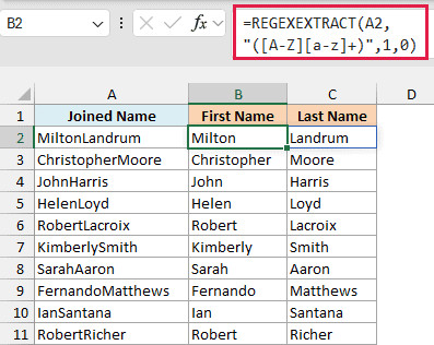
The above formula looks for the pattern ([A-Z][a-z]+), which means that it looks for all the matching strings that start with an uppercase letter followed by all the lowercase letters.
In our example, it finds two pattern matches, the first and the last name, and it then gives us the result in two separate cells.
So, I can just enter this one formula in the cell and drag it down, and it will give me the first as well as the last name in two separate cells.
Also read: How to Switch First and Last Name in Excel with Comma?
Example 3 – Extract Username/Domain from Email
Below, I have a dataset where I have email addresses in column A, and I want to get the username and the domain name in separate columns.
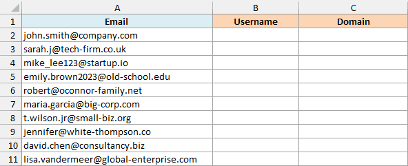
Again, while there are other ways to do this in Excel, let me show you how to do this using REGEX.
Here is the formula to get the username from email using the REGEXEXTRACT function:
=REGEXEXTRACT(A2:A11, "^([^@]+)")
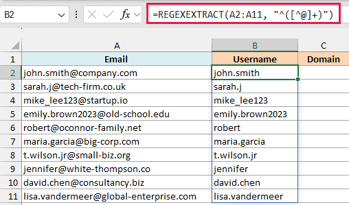
In this regex pattern:
- ^ – Matches the start of the string
- ( – Starts a capturing group
- [^@]+ – Matches one or more characters that are not ‘@’
- ) – Ends the capturing group
This pattern will capture everything from the start of the string up to (but not including) the ‘@’ symbol, which is typically the username in an email address.
And if you want to get the domain name, you can use the below formula:
=REGEXEXTRACT(A2:A11, "[^@]+$")
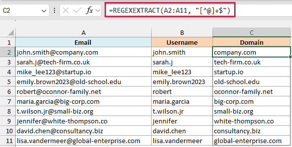
In this regex pattern:
- [^@] – This is a negated character set and matches any character that is not an @ symbol.
- + – This quantifier means “one or more of the preceding element”. So [^@]+ means “one or more characters that are not @”.
- $ – This gives us the matching string from the end of the text in the cell.
For known valid email addresses, TEXTBEFORE and TEXTAFTER are simpler in Microsoft 365 or Excel 2024. These regex examples teach negated character classes; they don’t validate addresses.
If you’re thinking this can easily be done with regular text formulas in Excel, have a look at the next example.
Example 4 – Extract Email from Text
Now, let’s dial up the complexity a little bit.
Below, I have a dataset where I have some text in column A, and I want to extract the email addresses from each cell.

Now, this is a bit complicated as the email can be anywhere in the text.
Here is the regex formula in Excel to tackle this:
=REGEXEXTRACT(A2:A11,"[A-Za-z0-9._%+-]+@[A-Za-z0-9.-]+\.[A-Za-z]{2,}")
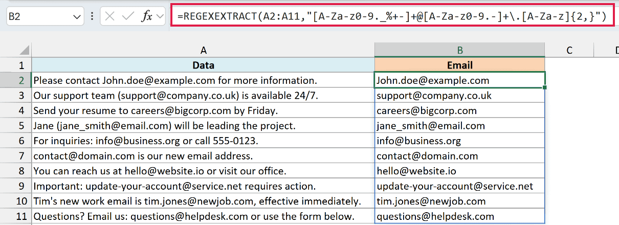
In this regex pattern:
- [A-Za-z0-9._%+-]+ – This matches one or more characters that can be:
- Uppercase letters (A-Z)
- Lowercase letters (a-z)
- Numbers (0-9)
- Special characters: . _ % + –
- @ – This matches the @ symbol, which is required in email addresses
- [A-Za-z0-9.-]+ – This matches one or more characters that can be:
- Uppercase letters (A-Z)
- Lowercase letters (a-z)
- Numbers (0-9)
- dot or hyphen
- \. – This matches a literal dot (.)
- [A-Za-z]{2,} – This matches two or more letters that can be:
- Uppercase letters (A-Z)
- Lowercase letters (a-z)
This extracts common ASCII email-shaped text, rather than validating every possible email address. A cell with no matching text returns an error.
While this works well if you only have one email address in the text, what if you have two or more?
Below, I have a dataset where I want to extract all the emails in the text in column A in column B (separated by a comma).

In this case, we can use a slightly modified regex pattern along with the TEXTJOIN function.
Here is the formula to do this:
=TEXTJOIN(", ", TRUE,REGEXEXTRACT(A2,"[A-Za-z0-9._%+-]+@[A-Za-z0-9.-]+\.[A-Za-z]{2,}", 1))
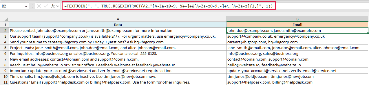
Enter this formula in cell B2 and then copy it for all the other cells in the column.
In the above formula, I have used 1 as the [return_mode] argument in the REGEXEXTRACT function. This gives me all the matching strings (which are all the email addresses).
And since I wrapped this REGEXEXTRACT formula in TEXTJOIN, it gives me all the email addresses in single cells separated by a comma.
Example 5 – Extract Text in Parentheses
Below, I have a data set where I have some text in column A, and I want to extract the first complete nonnested pair of parentheses into column B, including the parentheses.

Here is the formula to do that:
=REGEXEXTRACT(A2:A11,"\([^()]*\)")
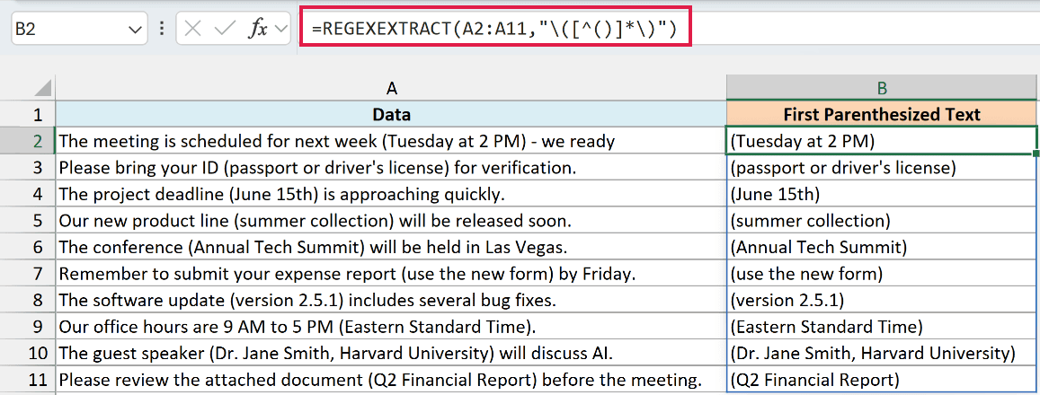
In the above formula’s regex pattern:
- \( – This matches a literal opening parenthesis.
- [^()]* – This matches zero or more characters that are not opening or closing parentheses.
- \) – This matches a literal closing parenthesis.
If you want to get the result without the parentheses, you can use the below formula:
=REGEXEXTRACT(A2:A11,"\(([^()]*)\)",2)
The third argument, 2, returns the captured content without its outer parentheses. Both formulas return the first complete nonnested pair, not every group or nested parentheses.
Example 6 – Extract Numbers from String
Extracting numbers from an alphanumeric string in Excel can be a complicated regular (non-regex) Excel formula.
But with regex, this is really simple.
Below, I have a data set where I have some data in column A, and I want to extract the numbers in the text in each cell into the adjacent cell in column B.

Here is the regex formula that does that:
=REGEXEXTRACT(A2:A6, "\d+")

This is so simple and one of my favorite examples to show the utility of regex.
In this regex pattern:
- \d – this represents any digit from 0 to 9
- + – this is a quantifier that means “one or more” of the preceding element (which is a digit).
So what this means is that this regex pattern is going to identify where a number starts in the text string, and it is going to keep going till it finds a non-digit character.
The default return_mode gives the first digit group from each cell as text. It doesn’t join separate groups or turn the result into a number.
And what if you have multiple numbers in the same cell (as shown below) and you want to extract all numbers in one cell?
You can use the following formula:
=TEXTJOIN(", ",TRUE,REGEXEXTRACT(A2, "\d+",1))

In the above formula, I have used REGEXEXTRACT(A2, “\d+”,1), where 1 is the third argument, return_mode. It extracts all the digit groups into separate cells.
The TEXTJOIN function then combines all the numbers and gives them in one cell (separated by a comma).
These patterns extract digit runs as text. Decimal points, minus signs, and thousands separators split groups, so this isn’t a general numeric-value parser.
Example 7 – Extract URLs from Text String
Below, I have some data in column A, and I want to extract only the URLs from this data in column B.

Here is the formula to do this:
=IFERROR(REGEXEXTRACT(A2:A6,
"\b(https?://[^\s]+|www\.[^\s]+)\b"),"URL Not Found")

In the above regex pattern:
- \b – This represents a word boundary. It ensures the pattern matches whole words, not parts of words.
- (…) – Parentheses group parts of the regex together.
- https?:// – this would match http:// as well as https://
- [^\s]+ – this would look for any character that is not whitespace and will continue to look till it finds a whitespace
- | – this is an OR operator, separating two alternatives
- www\. – this matches “www.” literally. The backslash makes the dot a literal character.
- [^\s]+ – this would look for any character that is not whitespace and will continue to look till it finds a whitespace
- \b – another word boundary to end the match
This extracts the first URL-like token. IFERROR shows “URL Not Found” for errors, including no match. It isn’t full URL validation, and surrounding punctuation can affect the match.
Example 8 – Get Phone Number in Specific Format
You can use the REGEXREPLACE function in Excel to find a pattern and replace it with something else.
This replacement could be a completely different string or a different format of the pattern REGEXREPLACE has found.
Below I have a data set where I have some phone numbers in different formats in column A, and I want them all in the standard (XXX) XXX-XXXX format.

Here is the formula to do this:
=REGEXREPLACE(REGEXREPLACE(A2:A9, "[^\d+]", ""),"^(\+?\d{0,3})?(\d{3})(\d{3})(\d{4})$","($2) $3-$4")

Let me explain how this works:
- REGEXREPLACE(A2:A9, “[^\d+]”, “”) – This part of the formula removes everything except digits and plus signs.
- ^(\+?\d{0,3})? – This optional prefix group starts at the beginning of the string. The question mark after the escaped plus sign makes that sign optional, and \d{0,3} allows up to three prefix digits.
- (\d{3})(\d{3})(\d{4})$ – this part of the pattern will create three groups of three digits, three digits, and four digits. The $ means that these need to be at the end, so the last ten digits are taken by this.
- ($2) $3-$4 – this is the part where we are replacing the identified three groups (in the above bullet point) and making them show up in the (XXX) XXX-XXXX format.
This formats the last ten matched digits and discards an optional prefix, including country codes. It doesn’t validate phone numbers or normalize international numbering.
If the cleaned string doesn’t match the pattern, REGEXREPLACE returns it unchanged.
Example 9 – Check Text Starting/Ending with a Specific Word
One common use case of REGEX is to check whether a string contains a specific word or not.
While this can be easily done in Excel with functions such as FIND or SEARCH, with the REGEXTEST function, you can take it up a notch.
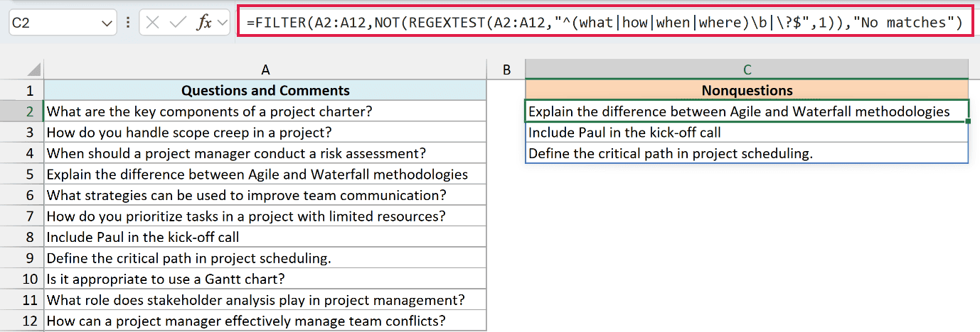
Below, I have a dataset where I have some questions and comments in column A, and I want to extract all the questions from this data.

Here is the formula that will do this:
=FILTER(A2:A12,REGEXTEST(A2:A12,"^(what|how|when|where)\b|\?$",1),"No matches")
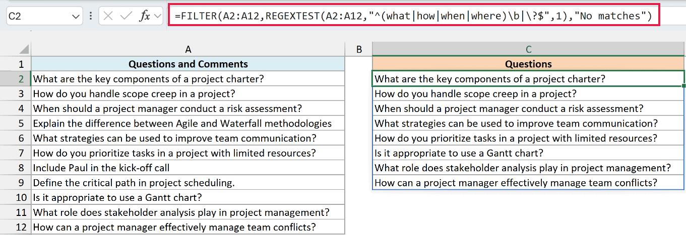
Use C2 as the output cell for either formula, with space below for the spill.
In the above formula, I have used a REGEXTEST function with the following pattern:
^(what|how|when|where)\b|\?$
The pattern flags text that starts with the whole word what, how, when, or where, or ends with a question mark. The 1 argument makes matching case-insensitive.
This is a simple question rule, not a general language test. Leading or trailing spaces can change which cells match.
The FILTER function returns the cells in column A where this question rule is TRUE.
In case you want to get all the cells where there is no question, you can use the below formula:
=FILTER(A2:A12,NOT(REGEXTEST(A2:A12,"^(what|how|when|where)\b|\?$",1)),"No matches")
Example 10 – Check if the String Contains Dates
Below, I have a data set where I have some cells that contain date-shaped text, and I want to use a regex pattern to find that text.

Here is the formula to do this:
=REGEXTEST(A2, "\d{2}[/.-]\d{2}[/.-]\d{4}")

The above formula returns TRUE when it finds text matching this date-shaped pattern, and FALSE when it doesn’t.
This pattern expects two digits, a slash, dot, or dash, two digits, another separator, and four digits. It doesn’t determine whether the day or month comes first.
It can also match invalid dates such as 99/99/2024 or mixed separators. Validate the date separately if you need a real Excel date.
You can modify the formula if there is any other date pattern you would like to include.
If you want to extract the first date-shaped text from each cell, you can use the below formula:
=IFERROR(REGEXEXTRACT(A2:A6, "\d{2}[/.-]\d{2}[/.-]\d{4}"), "No date found")
Example 11 – Check If String Contains Specific Words
Below, I have a data set, and I want to check whether the cells contain Python, JavaScript, or both.

Here is the formula to do this:
=REGEXTEST(A2:A6, "Python|JavaScript")

In the above formula, the pipe in Python|JavaScript is an OR operator. It checks whether Python, JavaScript, or both appear anywhere in the cell.
The default match is case-sensitive and substring-based, so it doesn’t require a whole word. Use a different pattern if you need word boundaries.
Here are some variations of the patterns you can use:
- ^(Python|JavaScript) – Starting with Python or JavaScript
- (Python|JavaScript)$ – Ending with Python or JavaScript
- (?i)Python|JavaScript – Case-insensitive match for Python or JavaScript
In this article, I showed you a couple of examples of using the new REGEX functions in Excel. To be honest, I’ve barely scratched the surface, and there are many more amazing things you can do with creating your own regex patterns.
If you have come across a useful example, I would love to hear about it in the comments section.
Other Excel articles you may also like:
