Paste into Filtered Column (Skipping Hidden Cells) in Excel

Excel is an amazing spreadsheet tool, but there are some things that drive me crazy.

One such thing is when you need to copy and paste data into a column with filtered rows.

Excel would paste this data into the visible cells as well as the hidden cells that have been filtered out. In most cases, this is not what you want.

In most cases, you want to paste your data only in the visible cells and not the hidden ones.

So how do we do this then?

In this article, I will show you a couple of workarounds for pasting into filtered columns in Excel while skipping the hidden cells.

Since there is no one solution that fits all, I will show you different scenarios and the most appropriate solution for each scenario (including a simple VBA code that works great).

Copy Paste One Single Cell Value in a Filtered Column

Let’s start with the most straightforward example.

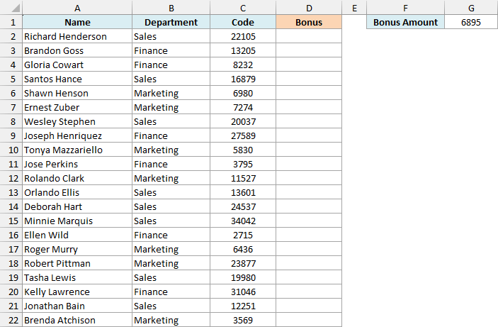
Below, I have a dataset that I am going to use (this is the One Value sheet in the example file).

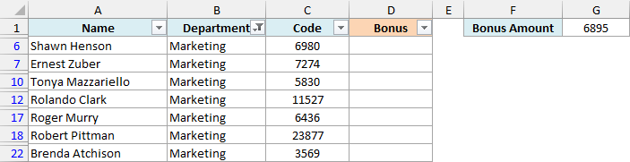
Now, I have filtered this data to only show the records for the Marketing department.

Now, I want to copy the value in cell G1 and paste the same in all the visible cells in column D (i.e., only the cells that are visible and not the ones that are hidden after filtering).

This is very easy, as you can simply copy the value in cell G1, then select all the cells in column D and paste it.

Here are the steps to do this:

1. Copy cell G1.

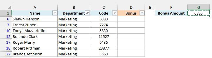
2. Select all the cells in column D in which you want to paste the value in G1.

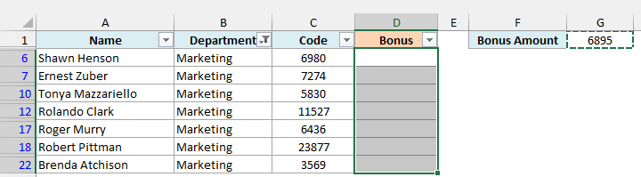
3. Use Control + V to paste the value.

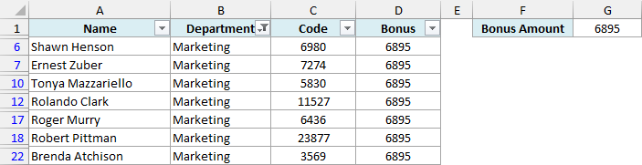
When I copied cell G1 and then selected cells in a column that has a filter applied to it, and then pasted the cell, it was only pasted in the cells that were visible.

You can confirm this by removing the filter, and you will notice that the value in cell G1 has only been pasted in the cells that were visible when the filter was applied.

This works here because I copied one single cell. When you copy a range of cells, Excel pastes into the hidden cells as well, as you will see in the next section.

Important: Use Control + V here and not Paste Values. If you use Paste Values on this selection (Control + Shift + V or the right-click menu), the value goes into the hidden cells as well.

In case you want to paste only the value (for example, when G1 has a formula), first select the cells in column D and then press ALT + semicolon to select only the visible cells. After that selection, Paste Values skips the hidden cells.

ALT + semicolon is the Windows shortcut. On a Mac, use Shift + Command + *.

Also read: Copy Visible Cells Only in Excel

Copy Paste Cells from the Same Row in a Filtered Column

Let’s look at another situation (which is not as straightforward).

Below, I have a filtered data set, and I have some values in column F that I want to copy and paste into the visible cells in column D (this is the Same Row Formula sheet in the example file).

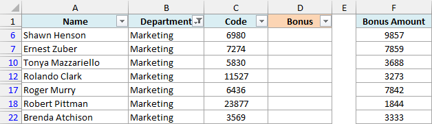
Now, you cannot do a simple copy and paste in this situation, as it won’t work.

If I copy the cells in column F, it is only going to copy the cells that are visible.

But if I then paste it in the cells in column D, it is going to paste it in the visible cells as well as the ones that are not visible.

So if you try it, you may end up getting a result as shown below.

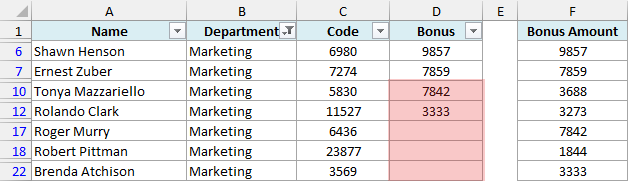
Also, if you think you can try selecting only the visible cells in column D (which you can do by using the shortcut ALT + semicolon) and then paste the values copied from column F, Excel will give you the following error.

Thankfully, when you have the values that you want to copy in the same row as your filter data set, you can use a very simple formula. The example file already has the finished formulas in column D.

Here are the steps to do this:

1. Select cell D6 (which is the first cell in our filtered data set in column D)

2. Enter an equal to sign

3. Select cell F6. This will make the reference in cell D6 as =F6.

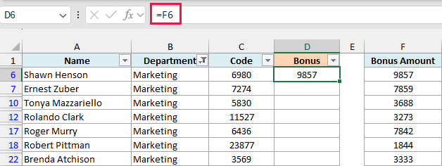
4. Press the Enter key

5. Copy the formula in all the cells in the column. You can do a simple copy-paste or drag the fill handle down to apply the formula to the entire column.

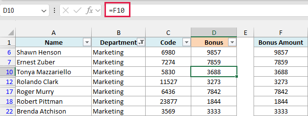
The good thing here is that when you copy and paste a formula in all the cells in a filtered dataset, it is only copied to the visible cells.

I am using a regular formula here (and in the other formula methods in this article) and not a spilling formula like =F2:F22.

A spilling formula is one formula in a single cell, like D2, whose results flow into the cells below it. That includes the hidden ones, which is exactly what we are trying to avoid.

Once you have the values in column D, you can convert the formula into values, and for that you need to remove the filter first.

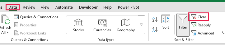
6. Click the Data tab and then click on Clear to remove the filter.

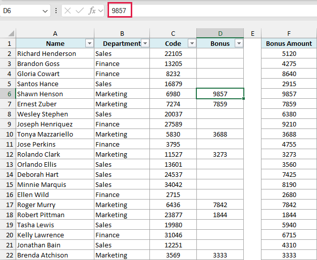
7. Select all the cells in column D (D2:D22 in our example), and then use Control + C to copy them.

8. Use Control + Shift + V to paste the formula as values. You can also right-click on the selected cells and then click on Paste Values.

Important: Do not try to paste the values with the filter still on. Excel shows an error saying that the Copy area and paste area aren’t the same size, and the formulas stay as they are.

Pasting the values over D2:D22 with the filter off doesn’t change the values already in the rows that were hidden, but any formulas in those rows become static values. If you need the filter back, you can apply it again after this.

Also read: How to Copy and Paste Column in Excel?

Paste into Visible Cells Only Using Fill Left

If you don’t want to use a formula for same-row values, the Fill option can do this directly, because it only fills the visible cells in a filtered column.

Below, I have the same filtered data set with values in column F, and I want to get these values into the visible cells in column D (this is the Same Row Fill sheet in the example file).

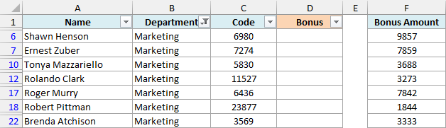
Here are the steps to do this:

1. Select the visible cells in column D by selecting D6:D22.

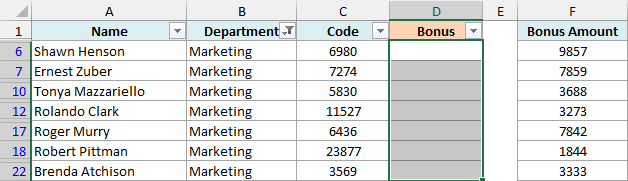
2. Hold the Control key and select F6:F22.

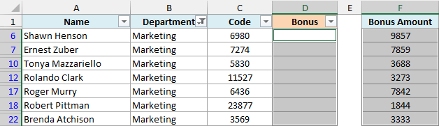
3. Click the Home tab, then click on Fill, and then click on Left.

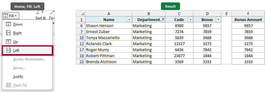
Excel copies the values from column F into the visible cells in column D. The hidden cells in column D stay as they were, and column E (which is between the two) doesn’t change.

If the values you want to copy are in a column to the left, select both columns the same way and use Control + R (the Fill Right shortcut).

Note that Fill copies the formatting of the cells along with their contents, so column D will pick up any number format or font style that column F has.

While these two methods work great, it’s likely that you may not get the data you want to copy and paste into the filtered rows in the same rows.

What if the data you want to copy and paste into the filtered rows is in a different location in the same worksheet or in a completely different worksheet or workbook?

The methods below would tackle that.

Copy Paste Cells From Another Range Sheet or Workbook into a Filtered Column

Below, I have a filtered data set.

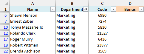
I also have some values on a different sheet (called Copy From) that I want to copy and paste into column D in our filter dataset above.

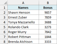
No copy-paste trick would work in this situation, so I have to get a bit creative. Formatting the data as an Excel Table doesn’t help either, as the pasted values still go into the hidden rows.

Now, there could be two situations.

1. There is a common column in both datasets that I can use to fetch the value from the Copy From sheet. For example, in our case, I can use the name column to look up each value and fetch it in the filter data set.
2. There is no common column, and I cannot use any lookup formulas

Let’s see what to do in both of these situations.

Using XLOOKUP or VLOOKUP (if there is a Lookup Value)

Let’s first take an example where I have the names column in both datasets, and I can use a lookup function (VLOOKUP or XLOOKUP) to fetch the value for each name in the filtered dataset.

Below is the filtered data on the Lookup sheet, and I want to get the bonus for each visible name from the Copy From sheet into column D (the example file already has the finished XLOOKUP formulas there).

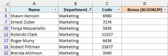
Below is the XLOOKUP formula that would work:

=XLOOKUP(A6,'Copy From'!$A$2:$A$8,'Copy From'!$B$2:$B$8)

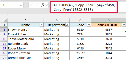
Enter this formula in cell D6 (or whatever is the first cell in the filtered column) and then copy it for all the other cells.

The formula looks for the name in A6 in the names on the Copy From sheet, and gives us the bonus next to it. Since it was copied into a filtered column, only the visible rows get the formula.

If a name isn’t on the Copy From sheet, the formula gives a #N/A error, so a missing name shows up instead of quietly turning into a blank cell.

The XLOOKUP function is available in Excel 365, Excel 2024, and Excel 2021.

If you are using Excel 2019 or earlier, enter the below VLOOKUP formula in the first visible cell and then copy it for all the other cells (the example file has it in column E):

=VLOOKUP(A6,'Copy From'!$A$2:$B$8,2,FALSE)

Once you have the formula results, you can convert these formulas into static values, and you’re done. Remove the filter first and then paste as values, the same way as in the same-row method.

Also read: Copy and Paste Multiple Cells in Excel (Adjacent & Non-Adjacent)

Paste a List into Visible Cells Only Using a Formula

Now let’s look at the situation where there is no common column, so I cannot use any lookup formulas.

Below is the filtered data on the List Formula sheet, and I want to get the values from the Bonus List sheet into column D (the example file already has the finished formulas there).

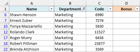
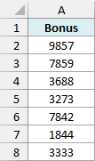
Here is the Bonus List sheet with the values that I want to bring in. Since there are no names to match on, these values need to already be in the same order as the visible rows.

Below is the formula that will do this:

=INDEX('Bonus List'!$A$2:$A$8,COUNTA(D$1:D5))

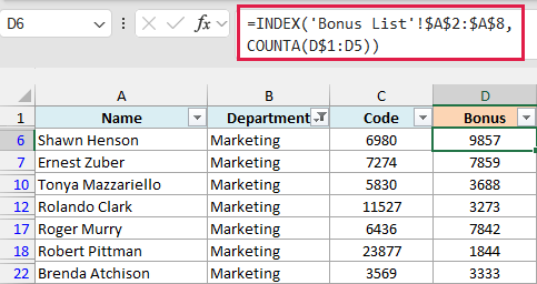
Enter this formula in cell D6 (the first visible cell in column D) and then copy it for all the other cells.

The range in the COUNTA function starts from the header in D1 and ends in the row just above the cell with the formula.

How this formula works:

• COUNTA(D$1:D5) counts the filled cells above the formula. In D6, that’s only the header in D1, so it gives us 1, and the INDEX function picks the first value from the list.
• In the next visible cell (D7), the range becomes D$1:D6. It now counts the header and D6, so it gives us 2, and the INDEX function picks the second value.
• The hidden cells in column D are empty, so they don’t get counted. That’s why the count goes up by one only for each visible row.

Important: This formula only works when the hidden cells in column D are empty and D1 has a header. If the hidden cells have data, you get wrong values or a #REF! error, so use the VBA method below instead.

You will also get the #REF! error in the last few cells if your list has fewer values than there are visible rows.

The COUNTA function doesn’t care about the filter, so the results stay the same when you remove it. So you can remove the filter and then paste as values, the same way as in the same-row method.

Using VBA (works in all scenarios)

Now, let’s talk about the most complicated situation (which is also perhaps the most common one).

I have the filtered data set below (this is the VBA sheet in the example file).

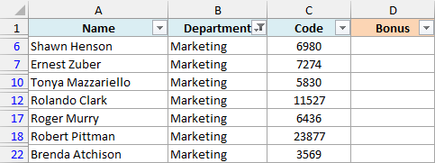
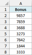
I have these values in a different worksheet or workbook (here it’s the Bonus List sheet), and I want to copy and paste them into column D in the filtered column.

There is no common column, so I cannot use any lookup formulas, and column D may already have data in its hidden cells, which rules out the COUNTA formula.

In such a case, I will have to rely on the big guns – a VBA macro code.

Below is the VBA macro code that would do this for me:

Sub PasteintoFilteredColumn()

    Dim visibleSourceCells As Range
    Dim destinationCells As Range
    Dim initialDestinationLastRow As Long
    Dim sourceCell As Range
    Dim destCell As Range
    Dim visibleDestinationCount As Long

    If Application.Selection.Cells.Count = 1 Then
        Set visibleSourceCells = Application.Selection
    Else
        Set visibleSourceCells = Application.Selection.SpecialCells(xlCellTypeVisible)
    End If

    On Error Resume Next
    Set destinationCells = Application.InputBox("Please select the destination cells:", Type:=8)
    On Error GoTo 0

    If destinationCells Is Nothing Then Exit Sub

    For Each destCell In destinationCells.Cells
        If destCell.EntireRow.Hidden = False Then visibleDestinationCount = visibleDestinationCount + 1
    Next destCell

    If visibleSourceCells.Cells.Count > visibleDestinationCount Then
        MsgBox "You are copying more cells than there are visible cells to paste into. Nothing was pasted."
        Exit Sub
    End If

    Application.ScreenUpdating = False

    initialDestinationLastRow = destinationCells.Rows(destinationCells.Rows.Count).Row

    For Each sourceCell In visibleSourceCells.Cells

        For Each destCell In destinationCells.Cells
            If destCell.EntireRow.Hidden = False Then

                sourceCell.Copy
                destCell.PasteSpecial Paste:=xlPasteValues

                If destCell.Row < initialDestinationLastRow Then
                    Set destinationCells = destCell.Offset(1, 0).Resize(initialDestinationLastRow - destCell.Row)
                End If

                Exit For
            End If

        Next destCell
    Next sourceCell

    Application.CutCopyMode = False
    Application.ScreenUpdating = True

End Sub

Sub PasteintoFilteredColumn()

    Dim visibleSourceCells As Range
    Dim destinationCells As Range
    Dim initialDestinationLastRow As Long
    Dim sourceCell As Range
    Dim destCell As Range
    Dim visibleDestinationCount As Long

    If Application.Selection.Cells.Count = 1 Then
        Set visibleSourceCells = Application.Selection
    Else
        Set visibleSourceCells = Application.Selection.SpecialCells(xlCellTypeVisible)
    End If

    On Error Resume Next
    Set destinationCells = Application.InputBox("Please select the destination cells:", Type:=8)
    On Error GoTo 0

    If destinationCells Is Nothing Then Exit Sub

    For Each destCell In destinationCells.Cells
        If destCell.EntireRow.Hidden = False Then visibleDestinationCount = visibleDestinationCount + 1
    Next destCell

    If visibleSourceCells.Cells.Count > visibleDestinationCount Then
        MsgBox "You are copying more cells than there are visible cells to paste into. Nothing was pasted."
        Exit Sub
    End If

    Application.ScreenUpdating = False

    initialDestinationLastRow = destinationCells.Rows(destinationCells.Rows.Count).Row

    For Each sourceCell In visibleSourceCells.Cells

        For Each destCell In destinationCells.Cells
            If destCell.EntireRow.Hidden = False Then

                sourceCell.Copy
                destCell.PasteSpecial Paste:=xlPasteValues

                If destCell.Row < initialDestinationLastRow Then
                    Set destinationCells = destCell.Offset(1, 0).Resize(initialDestinationLastRow - destCell.Row)
                End If

                Exit For
            End If

        Next destCell
    Next sourceCell

    Application.CutCopyMode = False
    Application.ScreenUpdating = True

End Sub

Here are the steps to put the VBA code in the backend in Excel:

1. Hold the ALT key and then press the F11 key. This will open the Visual Basic editor in the workbook. You can also do the same thing by clicking on the Developer tab and then clicking on the Visual Basic icon.

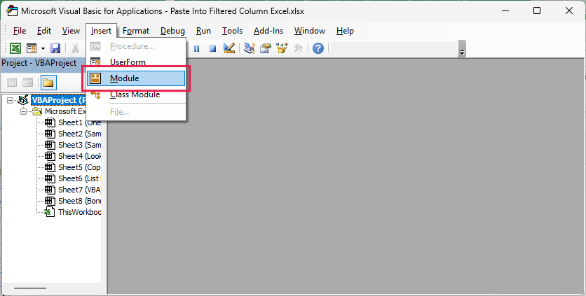
2. In the VB Editor, click on the Insert option in the menu and then click on Module. This will insert a new module where we will copy and paste the above VBA macro code.

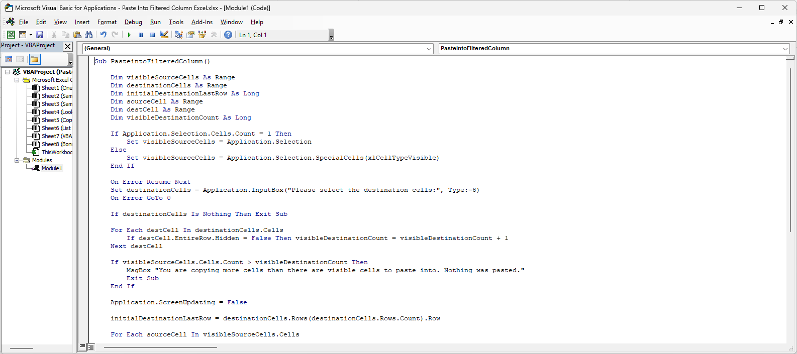
3. Copy and paste the above VBA code into the Module code window.

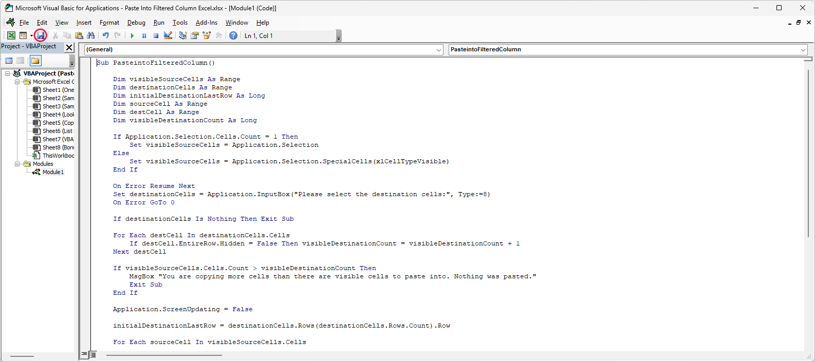
4. Click on the Save icon and close the VB editor. If your workbook is a regular .xlsx file, save it as a macro-enabled .xlsm file, or the code won’t be saved with it.

The example file is a regular .xlsx file, so it doesn’t have this code in it, and you will need to add it using the above steps.

Important: Remember that the changes done by a VBA code cannot be undone, so it’s always a good idea to keep a backup copy of your data set.

Now that we have the VBA code in place, below are other steps to use it to copy data into the filtered data set while skipping the hidden cells:

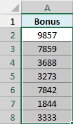
1. Select the cells that you want to copy and paste.

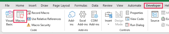
2. Click the Developer tab and then click on the Macros icon. This will open the Macros dialog box. If you don’t have the Developer tab, you can also use the keyboard shortcut ALT + F8.

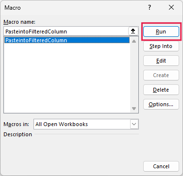
3. Select the PasteintoFilteredColumn macro and then click on Run.

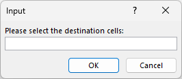
4. It will show you an input message box asking you to select the destination cells where you want to paste these selected data.

5. Navigate to the filtered data and select the cells where you want to paste the previously selected data.

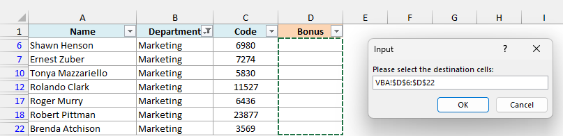
6. Click OK

As soon as you click OK, the magic behind the screen begins, and VBA pastes the data only into the visible filtered cells.

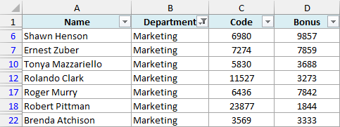
The code goes through the cells you selected in step 1 one by one and pastes each value into the next visible cell in the destination. It pastes values only, so the formatting of your source cells doesn’t come along.

If you select more cells in step 1 than there are visible cells in the destination (for example, when you pick only one destination cell), the code shows a message and pastes nothing. If you select fewer, only the first few visible cells get filled.

Also read: How to Select Entire Column (or Row) in Excel – Shortcut

Use Google Sheets to Paste into Filtered Column

And finally, if you’re ok with putting your data in Google Sheets, then you don’t need any special tricks or formulas or VBA code.

Regular copy-paste is going to work in Google Sheets.

Let me show you how it works.

Below, I have the same filtered data set in Google Sheets.

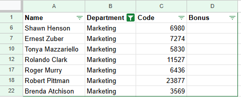
In another sheet, I have these values in a column that I want to copy and paste into column D in my filter data set.

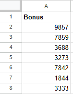
Here is how it works in Google Sheets:

1. Copy the data that you want to paste (you can use Control + C).

2. Select the filtered column range in which you want to paste this data

3. Paste the Data (use Control + V)

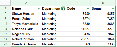
And that’s it – it’s that simple.

When it comes to pasting data in filtered rows, Excel and Google Sheets work differently. While Excel pastes a copied range into all the cells, whether visible or not, Google Sheets only pastes the data in the visible cells.

So, if it is possible for you to convert your Excel file into a Google Sheets or copy-paste data into a Google Sheets, then get the copy-paste done, and then bring the data back into Excel, you can also use this method.

Note that by default, there are only 1000 rows in Google Sheets. If your data set is bigger than that, Google Sheets adds the extra rows when you paste it in.

So these are some of the methods you can use to paste data into filtered column while skipping the hidden cells.

While I wish this were the default behavior in Excel, I hope the methods covered in this article help you get this done easily.

I hope you found this article helpful. In case you have any questions or you know of a method that can be used that I should have covered, do let me know in the comments section.

Other Excel articles you may also like:

• Highlight Active Row and Column in Excel (VBA)
• How to Count Filtered Rows in Excel?
• Dynamic Excel Filter Search Box – Extract Data as you Type
• Delete Rows Based on a Cell Value (or Condition) in Excel
• Excel VBA Autofilter: A Complete Guide with Examples
• How to Apply Formula to Entire Column in Excel (8 Easy Ways)