How to Reference Another Sheet or Workbook in Excel (with Examples)

To be able to reference cells and ranges is what makes any spreadsheet tool work. And Excel is the best and most powerful one out there.

In this tutorial, I will cover all that you need to know about how to reference cells and ranges in Excel. Apart from the basic referencing on the same sheet, the major part of this tutorial would be about how to reference another sheet or workbook in Excel.

While there is not much difference in how it works, when you reference another sheet in the same file or reference a completely separate Excel file, the format of that reference changes a bit.

Also, there are some important things you need to keep in mind when referencing another sheet or other external files.

But worry… nothing too crazy!

By the time you’re done with this tutorial, you will know all there is to know about referencing cells and ranges in Excel (be in the same workbook or another workbook).

Let’s get started!

Referencing a Cell in the Same Sheet

This is the most basic level of referencing where you refer to a cell on the same sheet.

For example, if I am in cell B1 and I want to refer to cell A1, the format would be:

=A1

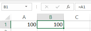
When you do this, the value in the cell where you use this reference will be the same as that in cell A1. And in case you make any changes in cell A1, these would be reflected in the cell where you have used this reference.

Referencing a Cell in the Another Sheet

If you have to reference another sheet in the same workbook, you need to use the below format:

Sheet_name!Cell_address

First, you have the sheet name followed by an exclamation sign which is followed by the cell reference.

So if you need to refer to cell A1 in Sheet 1, you need to use the following reference:

=Sheet1!A1

And if you want to refer to a range of cells in another sheet, you need to use the following format:

Sheet_name!First_cell:Last_cell

So, if you want to refer to the range A1:C10 in another sheet in the same workbook, you need to use the below reference:

=Sheet1!A1:C10

Note that I have only shown you the reference to the cell or the range. In reality, you would be using these in formulas. But the format of the references mentioned above are going to remain the same

In many cases, the worksheet you refer to would have multiple words in the name. For example, it could be Project Data or Sales Data.

In case you have spaces or non-alphabetical characters (such as @, !, #, -,etc.), you need to use the name within single quotes.

For example, if you want to refer cell A1 in the sheet named Sales Data, you will use the below reference:

='Sales Data'!A1

And in case the name of the sheet is Sales-Data, then to refer to cell A1 in this sheet, you need to use the below reference:

='Sales-Data'!A1

When you refer to a sheet in the same workbook, and then later change the name of the worksheet, you don’t need to worry about the reference breaking down. Excel will automatically update these references for you.

While it’s great to know the format of these references, in practice, it’s not such a good idea to manually type these every time. It would be time-consuming and highly error-prone.

Let me show you a better way to create cell references in Excel.

Also read: How to Sum Across Multiple Sheets in Excel?

Automatically Creating Reference to Another Sheet in the Same Workbook

A much better way to create cell reference to another sheet is to simply point Excel to the cell/range to which you want to create the reference and let Excel create it itself.

This will ensure that you don’t have to worry about the exclamation point or quotes being missing or any other format issue cropping up. Excel will automatically create the correct reference for you.

Below are the steps to automatically create a reference to another sheet:

1. Select the cell in the current workbook where you need the reference
2. Type the formula till you need the reference (or an equal-to sign if you just want the reference)
3. Select the sheet to which you need to refer to
4. Select the cell/range that you want to refer to
5. Hit Enter to get the result of the formula (or continue working on the formula)

The above steps would automatically create a reference to the cell/range in another sheet. You will also be able to see these references in the formula bar. Once you’re done, you can simply hit the enter key and it will give you the result.

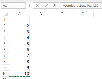
For example, if you have some data in cell A1:A10 in a sheet named Sales Data, and you want to get the sum of these values in the current sheet, following will be the steps:

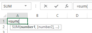
1. Type the following formula in the current sheet (where you need the result): =Sum(
2. Select the ‘Sales Data’ sheet.
3. Select the range that you want to add (A1:A10). As soon as you do this, Excel will automatically create a reference to this range (you can see that in the formula bar)
4. Hit the enter key.

When you’re creating a long formula, you may need to refer to a cell or a range in another sheet, and then have a need to come back to the origin sheet and refer to some cell/range there.

When you do this, you will notice that Excel automatically inserts a sheet reference to the sheet where you have the formula. While this is alright and doesn’t harm, it’s not needed. In such a case, you can choose to keep the reference or remove it manually.

Another thing you need to know when creating references by selecting the sheet and then the cell/range is that Excel will always create a relative reference (i.e., references with n0 $ sign). This means that if I copy and paste the formula (one with reference to another sheet) in some other cell, it would automatically adjust the reference.

Here is an example that explains relative references.

Suppose I use the following formula in cell A1 in current sheet (to refer to cell A1 in a sheet name SalesData)

=SalesData!A1

Now, if I copy this formula and paste in cell A2, the formula will change to:

=SalesData!A1

This happens because the formula is relative and when I copy and paste it, the references will automatically adjust.

In case I want this reference to always refer to cell A1 in the SalesData sheet, I will have to use the below formula:

=SalesData!$A$1

The dollar sign before the row and column number lock these references so that these don’t change.

Here is a detailed tutorial where you can learn more about absolute, mixed, and relative references.

Now that we have covered how to reference another sheet in the same workbook, let’s see how we can refer to another workbook.

How to Reference Another Workbook in Excel

When you refer to a cell or a range to another Excel workbook, the format of that reference would depend on whether that workbook is open or closed.

And of course, the name of the workbook and the worksheets also play a role in determining the format (depending on whether you have spaced or non-alphabetical characters in the name or not).

So let’s see the different formats of external references to another workbook in different scenarios.

External Reference to an Open Workbook

When it comes to referring to an external open workbook, you need to specify the workbook name, the worksheet name, and the cell/range address.

Below is the format you need to use when referring to an external open workbook

='[FileName]SheetName!CellAddress

Suppose you have a workbook ‘ExampleFile.xlsx’ and you want to refer to cell A1 in Sheet1 of this workbook.

Below is the reference for this:

=[ExampleFile.xlsx]SalesData!A1

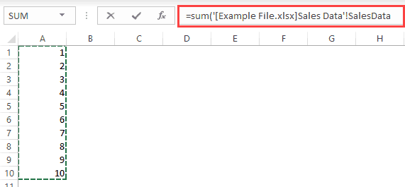
In case there are spaces in the external workbook name or the sheet name (or both), then you need to add put the file name (in square brackets) and the sheet name in single quotes.

Below are the examples where you would need to have the names in single quotes:

='[Example File.xlsx]SalesData'!A1

='[ExampleFile.xlsx]Sales Data'!A1

='[Example File.xlsx]Sales Data'!A1

How to Create Reference to Another Workbook (Automatically)

Again, while it’s good to know the format, it’s best not to type it manually.

Instead, just point Excel in the right direction and it will create these references for you. This is a lot faster with way fewer chances of errors.

For example, if you have some data in cell A1:A10 in a workbook named ‘Example File’ in the sheet named ‘Sales Data’, and you want to get the sum of these values in the current sheet, following will be the steps:

1. Type the following formula in the current sheet (where you need the result): =Sum(
2. Go to the ‘Example File’ workbook
3. Select the ‘Sales Data’ sheet.
4. Select the range that you want to add (A1:A10). As soon as you do this, Excel will automatically create a reference to this range (you can see that in the formula bar)
5. Hit the enter key.

This would instantly create the formula with the correct references.

One thing you would notice when creating a reference to an external workbook is that it will always create absolute references. This means that there is a $ sign before the row and column numbers. This means that if you copy and paste this formula to other cells, it would keep referring to the same range due to absolute reference.

In case you want this to change, you need to change the references manually.

External Reference to a Closed Workbook

When an external workbook is open and you refer to this workbook, you just need to specify the file name, sheet name, and the cell/range address.

But when this is closed, Excel has no clue where you look for the cells/range you referred to.

This is why when you create a reference to a closed workbook, you also need to specify the file path.

Below is a reference that refers to cell A1 in the Sheet1 worksheet in the Example File workbook. Since this file is not open, it also refers to the location where the file is saved.

='C:\Users\sumit\Desktop\[Example File.xlsx]Sheet1'!$A$1

The above reference has the following parts:

• File Path – the location on your system or network where the external file is located
• File Name – the name of the external workbook. This would include the file extension as well.
• Sheet Name – the name of the sheet in which you are referring to the cells/ranges
• Cell/Range Address – the exact cell/range address to which you’re referring

When you create an external reference to an open workbook and then closed the workbook, you would notice that the reference automatically changes. After the external workbook is closed, Excel automatically inserts a reference to the file path as well.

Impact of Changing File Location on References

When you create a reference to a cell/range in an external Excel file and then close it, the reference now uses the file path as well.

But then if you change the file location, nothing is going to change in your workbook (in which you create the reference). But since you have changed the location, the link has now been broken.

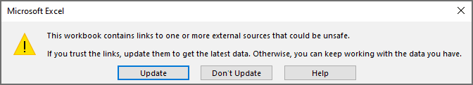
So if you close and open this workbook, it will tell you that the link is broken and you need to either update the link or break it completely. It will show you a prompt as shown below:

When you click on Update, it will show you another prompt where you can choose the options to edit the links (which will show you the below dialog box)

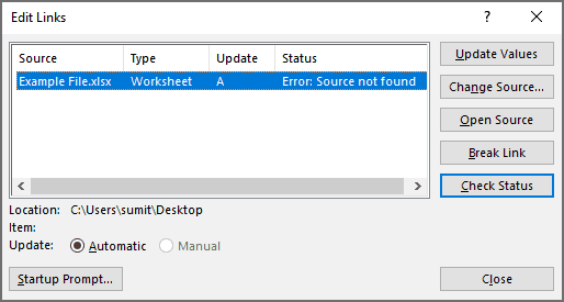
If you need to keep these files linked, you can specify the new location of the file by clicking on Update Values. Excel opens a dialog box for you where you can specify the new file location by navigating there and selecting it.

Reference to a Defined Name (in the same or external workbook)

When you have to refer to cells and ranges, a better way is to create defined names for the ranges.

This is helpful as it makes it easy for you to refer to these ranges using a name instead of a long and complicated reference address.

For example, it’s easier to use =SalesData instead of =[Example File.xlsx]Sheet1′!$A$1:$A$10

And in case you have used this defined named in multiple formulas and you need to change the reference, you need to only do it once.

Here are the steps to create a named range for a range of cells:

1. Select all the cells that you want to include in the named range
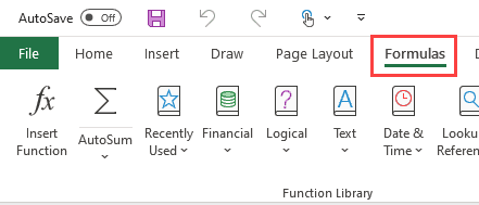
2. Click the Formulas tab
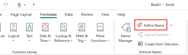
3. Click on the Define Name option (it’s in the Defined Names group)
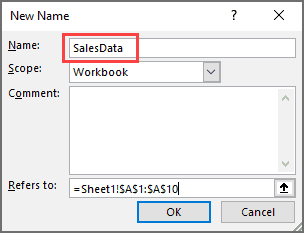
4. In the New Name dialog box, give this range a name (I am using the name SalesData in this example). Remember you can’t have spaces in the name
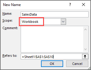
5. Keep the scope as Workbook (unless you have a strong reason to make it sheet-level)
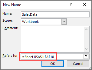
6. Make sure the Refers to the range is correct.
7. Click OK.

Now your named range has been created and you can use it instead of the cell references with cell addresses.

For example, if I want to get the sum of all these cells in the SalesData range, you can use the below formula:

=SUM(SalesData)

And what if you want to use this named range is other worksheets or even other workbooks?

You can!

You just need to follow the same format we have discussed in the above section.

No need to go back to the beginning of this article. Let me give you all the examples here itself so you get the idea.

Referencing the defined name in the same worksheet or workbook

If you have created the defined name for the workbook level, you can use it anywhere in the workbook by just using the defined name itself.

For example, if I want to get the sum of all the cells in the named range we created (SaledData), I can use the below formula:

=SUM(SaledData)

In case you have created a worksheet level named range, you can use this formula only if the named range is created in the same sheet where you’re using the formula.

In case you want to use it on another sheet (say Sheet2), you need to use the following formula:

=SUM(Sheet1!$A$1:$A$10)

And in case there are spaces or alphanumeric characters in the sheet name, you will have to put the sheet name in single quotes.

=SUM('Sheet 1'!$A$1:$A$10)

Referencing the defined name in another workbook (Open or Closed)

When you want to reference a named range in another workbook, you will have to specify the workbook name and then the name of the range.

For example, if you have an Excel workbook with the name ExampleFile.xlsx and a named range with the name SalesData, then you can use the below formula to get the sum of this range from another workbook:

=SUM(ExampleFile.xlsx!SalesData)

In case there are spaces in the file name, then you need to use these in single quotes.

=SUM('Example File.xlsx'!SalesData)

In case you’ve sheet-level named ranges, then you need to specify the name of the workbook as well as the worksheet when referencing it from an external workbook.

Below is an example of referencing a sheet-level named range:

=SUM('[Example File.xlsx]Sheet1'!SalesData)

As I mentioned above as well, it’s always best to create workbook level named ranges, unless you have a strong reason to create a worksheet level one.

In case you’re referencing a named range in a closed workbook, you will have to specify the file path as well. Below is an example of this:

=SUM('C:\Users\sumit\Desktop\Example File.xlsx'!SalesData)

When you create a reference to a named range in an open workbook and then close the workbook, Excel automatically changes the reference and adds the file path.

How to Create Reference to a Named Range

If you create and work with a lot of named ranges, it’s not possible to remember each one’s name.

Excel helps you by showing you a list of all the named ranges that you have created and allows you to insert these in formulas with a single click.

Suppose you have created a named range SalesData which you want to use in a formula to SUM all the values in the named range.

Here are the steps to do this:

1. Select the cell in which you want to enter the formula.
2. Enter the formula to the point where you need the named range to be inserted
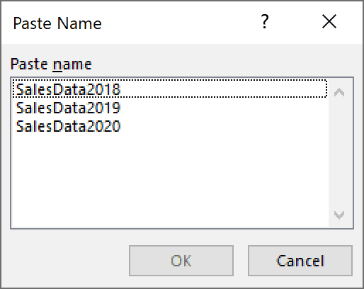
3. Hit the F3 key on your keyboard. This will open the Paste Name dialog box with the list of all the names you have created
4. Double-click on the name that you want to insert.

The above steps would insert the name in the formula and you can continue to work on the formula.

This is all you need to know about how to reference other sheets or workbooks and how to create an external reference in Excel.

Hope you found this tutorial useful.

You may also like the following Excel tutorials:

• How to Sum a Column in Excel
• CONCATENATE Excel Range (with and without separator)
• Hyperlinks in Excel (A Complete Guide + Examples)
• How to Find External Links and References in Excel
• How to Copy and Paste Formulas in Excel without Changing Cell References
• How to Delete Named Range in Excel?
• Using A1 or R1C1 Reference Notation in Excel (& How to Change These)