How to Calculate Number of Weeks Between Two Dates in Excel

When working with dates and making project plans in Excel, you may come across a situation where you want to know how many weeks there are between two dates.

While there is no built-in function to do this in Excel, this can easily be done using other simple functions.

In this article, I will show you how to calculate the number of weeks between two dates in Excel. I’ll also cover completed weeks, weeks and days, weeks to today, working weeks, and calendar weeks.

DAYS Function to Get Weeks Between Two Dates

A week always has seven days, so if we can find the total number of days between two given dates, we can easily find the total number of weeks by dividing this value by 7.

If you already have the number of days in a cell, simply divide that cell by 7. The formulas below are for when you only have the two dates.

Below, I have a list of home projects with the start date in column B and the end date in column C, and I want to calculate the total number of weeks between these two dates in column D.

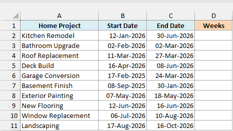
Here is the formula that will do this:

=DAYS(C2:C11,B2:B11)/7

I entered this formula in cell D2, and the results spill down to D11 automatically.

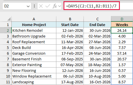
DAYS function subtracts the start date from the end date to give us the total number of days between these two given dates.

This value is then divided by 7 to get the total number of weeks between the two dates.

If you are using Excel 2019 or earlier, the above formula won’t spill, so enter the below formula in cell D2 and then copy it down the range:

=DAYS(C2,B2)/7

In case you see dates in column D instead of numbers, select the results, click the Home tab, then in the Number group, click on the Format drop-down and select General.

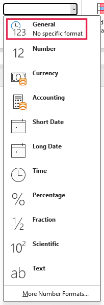
The General format will show more decimal places than you see here, because I’ve formatted these results to show two decimals.

As you must have already noticed, some of the results have decimal values (such as 24.14 in cell D2). In this case, 24 gives us the total number of completed weeks between these two dates.

The decimal portion is the part of a week that’s left over. Here, 0.14 of a week is 1 additional day after 24 weeks, and I’ll show you how to get those days as a number later in this article.

In case you only want to get the number of completed weeks, you can use the below formula in cell E2:

=INT(DAYS(C2:C11,B2:B11)/7)

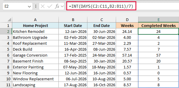
This will remove the decimal portion and only give you the integer part of the result.

If your end date comes before your start date, the result is negative, so a negative number usually means your dates are in the wrong columns.

Also, the INT function rounds a negative number away from zero, so -1.43 weeks becomes -2 and not -1.

In case you want to round up the value and count any decimal part as a complete week, you can use the formula below in cell F2:

=ROUNDUP(DAYS(C2:C11,B2:B11)/7,0)

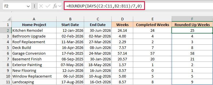
Important: The result you get is not inclusive of both the start date and the end date. For example, if your project starts on 1st January and ends on 11th January, the DAYS function would return 10.

If you want the start date and the end date to be included in the counting of days, you need to add 1 to the result of the DAYS function. Here is the formula I used in cell G2:

=(DAYS(C2:C11,B2:B11)+1)/7

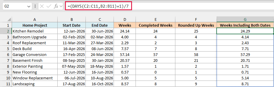
If you are using Excel 2019 or earlier, the formulas in cells E2, F2, and G2 work the same way as the older formula I showed earlier. Replace C2:C11 with C2 and B2:B11 with B2, then copy the formula down the range.

Also read: How to Add Week to Date in Excel?

Subtract Dates to Get Weeks Between Two Dates

Since dates are stored as serial numbers in Excel, you can also do a simple subtraction to get the number of days between two given dates and then calculate the number of weeks from that.

Below, I have a list of home projects with the start date in column B and the end date in column C, and I want to calculate the number of weeks between these two dates in column D.

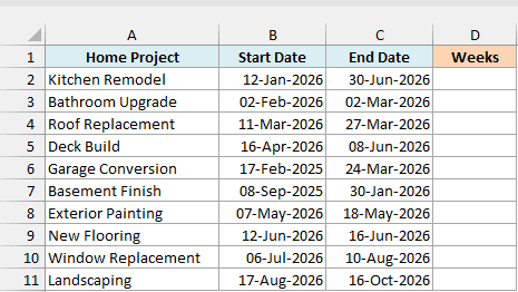
Here is the simple subtraction formula to do this:

=(C2:C11-B2:B11)/7

Enter this formula in cell D2, and the results spill down to D11 automatically.

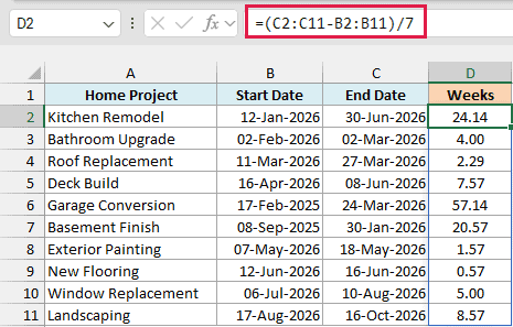
If you are using Excel 2019 or earlier, the above formula won’t spill, so enter the below formula in cell D2 and then copy it down the range:

=(C2-B2)/7

In case you only want to get the number of completed weeks, you can use the below formula in cell E2:

=INT((C2:C11-B2:B11)/7)

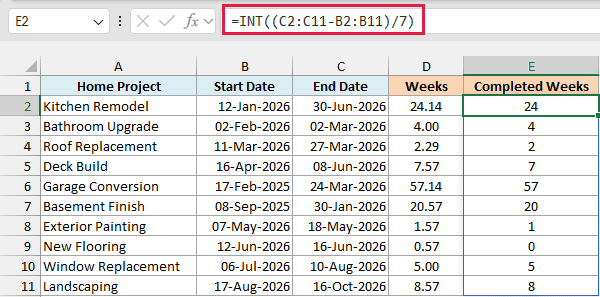
If you are using Excel 2019 or earlier, the formula in cell E2 works the same way as the older formula above. Replace C2:C11 with C2 and B2:B11 with B2, then copy the formula down the range.

Important: For this method to work, your dates need to be in a format that Excel recognizes as a valid date format and it shouldn’t be in the text format.

In some cases, when your date is in the text format, this formula may return a VALUE error.

Excel can still calculate text that it reads as a date, like 2026-01-12, but text it can’t read gives you the error. The DAYS function has the same problem, so switching to it won’t fix this.

A blank date causes a different problem, because you won’t get an error at all. Excel treats the blank cell as 0, so a missing start date gives you thousands of weeks, which is your clue to fill in the date.

Subtraction also counts any time stored with your dates, and the DAYS function doesn’t. If a project starts at 6 PM on one day and ends at 6 AM two weeks later, subtraction gives you 1.93 weeks, while the DAYS function gives you 2.

So use the DAYS function when only the dates matter, and subtraction when the hours should count too.

You may also come across the DATEDIF function for this, as in =DATEDIF(B2,C2,"d")/7. It has no unit for weeks, so you still need to divide by 7, and it returns a #NUM! error if the end date comes before the start date.

Also read: Get the Number of Days in a Month in Excel

Get Weeks and Days Between Two Dates

A result like 24.14 weeks isn’t always easy to read. Sometimes it’s more useful to show it as 24 weeks and 1 day, so let’s split the result into those two parts.

Below, I have a list of home projects with the start date in column B and the end date in column C, and I want the completed weeks in column D, the extra days in column E, and both together as text in column F.

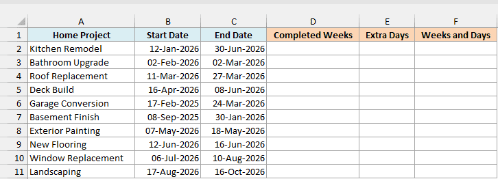
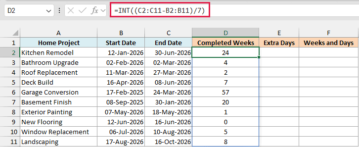
Here is the formula for the completed weeks, which I entered in cell D2:

=INT((C2:C11-B2:B11)/7)

And here is the formula for the extra days, which I entered in cell E2:

=MOD(C2:C11-B2:B11,7)

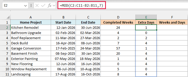
The MOD function gives you what’s left after dividing by 7. For example, the Kitchen Remodel runs for 169 days, which is 24 complete weeks with 1 day left over.

If you want both parts together in one cell, use the below formula in cell F2:

=LET(d,C2:C11-B2:B11,w,INT(d/7),r,MOD(d,7),w&IF(w=1," week "," weeks ")&r&IF(r=1," day"," days"))

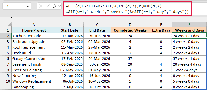
How this formula works:

• d,C2:C11-B2:B11 calculates the number of days and names that result d, so the formula doesn’t have to repeat it.
• w,INT(d/7) gets the completed weeks and names them w.
• r,MOD(d,7) gets the leftover days and names them r.
• w&IF(w=1," week "," weeks ")&r&IF(r=1," day"," days") joins everything into one text result. The two IF functions make sure you get “1 week” and “1 day” instead of “1 weeks” and “1 days”.

The LET function works in Excel 365 and Excel 2021 or later.

If you are using Excel 2019 or earlier, enter the below simpler formula in cell F2 and then copy it down the range (it will show “1 weeks” and “1 days” where those apply):

=INT((C2-B2)/7)&" weeks "&MOD(C2-B2,7)&" days"

The completed weeks and extra days formulas in cells D2 and E2 also work in older versions. Replace C2:C11 with C2 and B2:B11 with B2, then copy the formula down the range.

Count Weeks From a Date to Today

If a project is still going on, you won’t have an end date to work with. In that case, you can use today’s date as the end date.

Below, I have a list of home projects with the start date in column B, and I want to calculate the number of weeks so far in column C.

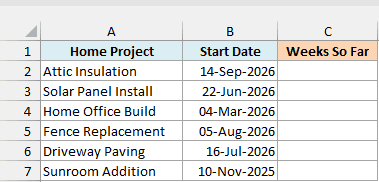
Here is the formula that will do this:

=(TODAY()-B2:B7)/7

Enter this formula in cell C2, and the results spill down to C7 automatically.

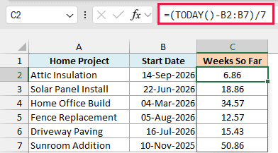
The TODAY function returns the current date, and it updates whenever the workbook recalculates. So the numbers grow every day, and the results you see in the example file will be different from the ones in this screenshot.

If you are using Excel 2019 or earlier, the above formula won’t spill, so enter the below formula in cell C2 and then copy it down the range:

=(TODAY()-B2)/7

In case you only want to get the number of completed weeks, you can use the below formula in cell D2:

=INT((TODAY()-B2:B7)/7)

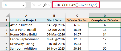
If you are using Excel 2019 or earlier, the formula in cell D2 works the same way as the older formula above. Replace B2:B7 with B2, then copy the formula down the range.

Calculate Working Weeks Between Two Dates

The methods so far count every day, including weekends. If you only care about the days people actually work, you can count weekdays and convert those into working weeks.

Below, I have a list of home projects with the start date in column B and the end date in column C, and I want to calculate the number of working weeks in column D.

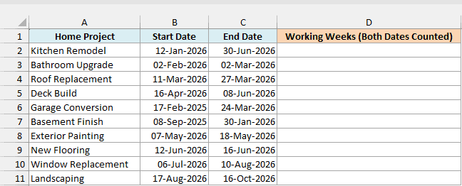
Here is the formula that will do this:

=NETWORKDAYS(B2:B11+0,C2:C11+0)/5

Enter this formula in cell D2, and the results spill down to D11 automatically.

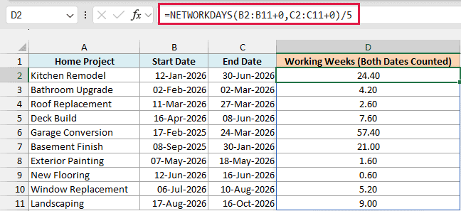
The NETWORKDAYS function counts the weekdays between the two dates, and dividing that count by 5 converts it into working weeks. For example, the Bathroom Upgrade has 21 working days, which gives you 4.20 working weeks.

NETWORKDAYS counts both the start date and the end date, unlike the formulas above. So the New Flooring project, which runs from a Friday to the following Tuesday, has 3 working days and shows 0.60.

You may have noticed the +0 in the formula. NETWORKDAYS returns a #VALUE! error when you give it plain ranges, and adding 0 turns each range into a list of date numbers it can work with, so the results spill.

This formula doesn’t know about your holidays, so they get counted as working days. The NETWORKDAYS function has a third argument for a holiday list, and the NETWORKDAYS.INTL function can handle a work week that doesn’t run from Monday to Friday.

If you are using Excel 2019 or earlier, the above formula won’t spill, so enter the below formula in cell D2 and then copy it down the range:

=NETWORKDAYS(B2,C2)/5

Count Calendar Weeks Between Two Dates

All the formulas so far measure how much time has passed. But a Friday and the following Tuesday are only 4 days apart and still fall in two different calendar weeks, so sometimes you need to count calendar weeks instead.

Below, I have a list of home projects with the start date in column B and the end date in column C, and I want the calendar weeks between the two dates in column D and the calendar weeks each project touches in column E.

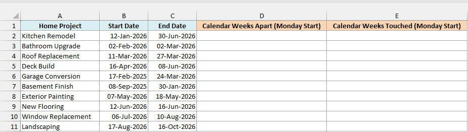
Here is the formula for the calendar weeks between the dates, which I entered in cell D2:

=(C2:C11-WEEKDAY(C2:C11,2)-(B2:B11-WEEKDAY(B2:B11,2)))/7

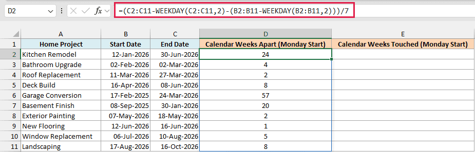
How this formula works:

• WEEKDAY(C2:C11,2) gives you the day number of each end date, where Monday is 1 and Sunday is 7.
• C2:C11-WEEKDAY(C2:C11,2) moves each end date back to the Sunday just before its week started, so every date in the same Monday to Sunday week lands on the same Sunday.
• B2:B11-WEEKDAY(B2:B11,2) does the same thing for the start dates.
• Subtracting one Sunday from the other and dividing by 7 tells you how many calendar weeks apart the two dates are.

For example, the New Flooring project runs from Friday, 12-Jun-2026 to Tuesday, 16-Jun-2026. That’s only 4 days, but the two dates are 1 calendar week apart.

This formula treats Monday as the first day of the week, because the 2 after the comma in each WEEKDAY function is what numbers Monday as 1. If your weeks start on Sunday, change that 2 to 1 in both WEEKDAY functions.

If you are using Excel 2019 or earlier, the above formula won’t spill, so enter the below formula in cell D2 and then copy it down the range:

=(C2-WEEKDAY(C2,2)-(B2-WEEKDAY(B2,2)))/7

In case you want to know how many calendar weeks a project touches, including the week it starts in, add 1 to the result. Here is the formula I used in cell E2:

=(C2:C11-WEEKDAY(C2:C11,2)-(B2:B11-WEEKDAY(B2:B11,2)))/7+1

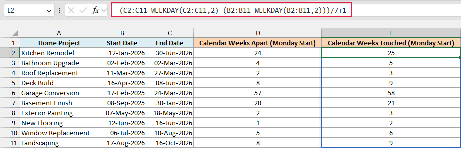
If you are using Excel 2019 or earlier, add 1 to the end of the older formula shown above, enter it in cell E2, and then copy it down the range.

Why the WEEKNUM Function Fails for Weeks Between Two Dates

You may also come across another way to calculate the number of weeks between two dates, which is using the WEEKNUM function. It looks like a smart shortcut, but it gives you wrong answers once the dates are more than 366 days apart.

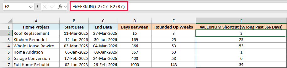
Below, I have a list of home projects, some longer than a year, with the start date in column B and the end date in column C, and I want to compare the WEEKNUM result in column F with the correct weeks in column E.

Column D has the number of days between the dates, and column E has the correct number of weeks, rounded up.

Here is the WEEKNUM formula:

=WEEKNUM(C2:C7-B2:B7)

Enter this formula in cell F2, and the results spill down to F7 automatically.

WEEKNUM Function works by taking the serial number of a date as input and giving us the week number of that date in that year.

However, in this example, we are using C2:C7-B2:B7 as the date serial number. Excel treats that number of days as a date counted forward from the start of 1900, so the week number works out to the weeks from the beginning of that year.

Also, note that this will always give you an integer value. It would automatically round up the result, so if there are 16 days, it would give you three weeks.

The problem starts after 366 days, because that “date” moves into 1901 and the week number starts again from 1. So 367 days gives you 1 and 400 days gives you 6, while column E correctly shows 53 and 58.

Important: Don’t use this WEEKNUM formula to count weeks, because it can give you a believable but wrong number with no error to warn you. Use =ROUNDUP((C2:C7-B2:B7)/7,0) instead, which is the formula in column E.

You may also see a formula that subtracts one week number from another, like =WEEKNUM(C2)-WEEKNUM(B2). This breaks when the two dates fall in different years because week numbers start again every January, so use the calendar weeks formula shown above instead.

These are some simple formula methods you can use to quickly calculate the number of weeks between two given dates.

I hope you found this article useful. If you know of any other method that can be used to do this, please share with us in the comments section.

Other Excel Articles You May Also Like:

• How to Autofill Only Weekday Dates in Excel (Formula)
• Excel WEEKDAY Function
• Check IF a Date is Between Two Given Dates in Excel
• Get Day Name from Date in Excel
• Convert Serial Numbers to Dates in Excel
• Convert Days to Months in Excel
• Calculate Number of Months Between Two Dates in Excel (Easy Formulas)
• How to Add or Subtract Days to a Date in Excel (Shortcut + Formula)
• Calculate Time in Excel (Time Difference, Hours Worked, Add/ Subtract)