
In the projects I have worked so far, Milestone Charts (also known as timeline charts) are often one of the most discussed parts.
A commitment to delivering is as important as the project itself. A milestone chart is an effective tool to depict project scope and timelines.
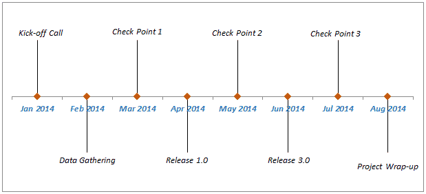
In this post, I will show you a simple technique to quickly generate a Milestone chart in Excel.
Something as shown below:
Steps to Create Milestone Chart in Excel
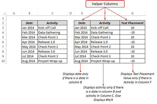
- Get the data in place. To create this, I have two columns of data (Date in B3:B10 and Activity in C3:C10) and three helper columns.
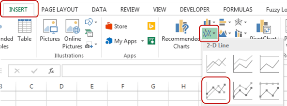
- Go to Insert –> Charts –> Line Chart with Markers
- Go to Design –> Select Data
- In Select Data Source dialogue box, click on Add
- In the Edit Series Dialogue box
- Series Name: Date
- Series Values: Activity Cells in Column F This inserts a line chart with X-Axis values as 1,2,3.. and Y-axis values as 0
- In the Select Data Source dialogue box, click on Edit in Horizontal (Category) Axis Labels and select dates in Column E. This changes X-Axis values to dates.

- In Select Data Source dialogue box, click on Add
- In the Edit Series Dialogue Box
- Series Name: Activity
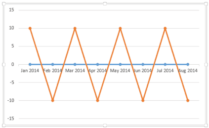
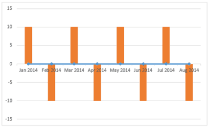
- Series Values: Text Placement Cells in Column G This inserts a haphazard line chart. Something as shown below:
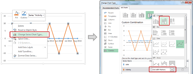
- Click on any of the Activity data-point, right-click and select a change chart type. In Change chart Type dialogue box, select the Column chart. This will change the haphazard Line chart into Column Chart
- This will change the haphazard Line chart into Column Chart
- In the Edit Series Dialogue Box
- Right-click on data bars and select Format Data Series. In series option pane, select
-
- Plot Series on: Secondary Axis This would introduce a secondary vertical axis on the right of the chart. Click on it and delete it.
-
- Go to Design –> Select Data
- In Select Data Source Dialogue box, select Activity series and click on Edit in Horizontal (Category) Axis Labels box. In the Axis Labels dialogue box, select Activity cells in column F
- Select bars, right-click and select Add Data Labels
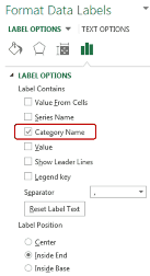
- Right-click on the data label and select Format Data Label
-
- In format data label pane, select Category Name (and un-check any other). This adds activity names as data labels. Adjust the position to get activity name at the tip of the bar
-
- Select and go to Design –> Add Chart Element –> Error Bars –> More Error Bar Options [For 2010, this option is in Layout –> Analysis]
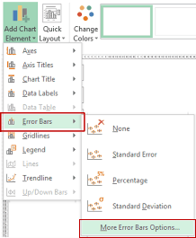
- In the Format Error Bars Pane, make the following selections
-
- Vertical Error Bar: Minus
- End Style: No Cap
- Error Amount: Percentage – 100%
-
- Right-click on bars and select Format Data Series. In Format Data Series Pane (in Fill and Line)
-
- Fill: No Fill
- Border: No Border
-
That’s it!! Your Milestone Chart is ready. Garnish it and serve it hot 🙂
Try it Yourself.. Download the file from here
You May Also Like the Following Excel Tutorials:
- Creating a Gantt Chart in Excel.
- Creating a Histogram in Excel.
- Excel Timesheet Calculator Template.
- How to Make a Pareto Chart in Excel.
- Employee Leave Tracker Template.
- Free Excel Templates Download.
- Creating a Bell Curve in Excel.
- Creating a Combination Chart in Excel.
- Creating an Area Chart in Excel.
- Advanced Excel Charts Examples.


Hello, this is just fantastic, love it. I was wondering if you knew (or if it was possible) to not include middle unused dates. I am making an evolutionary timeline, so jumping 100’s of millions of years is going to make the graph rather long..
Thanks!
Thanks sr, very nice and helpful for my project.
If it’s messing up when you add new data entries, make sure everything is sorted according to date.
Hi Sumit, what would the steps be to create a timeline like the first one shown, but using Excel for Mac 2011? My dialogue boxes are very different from your instructions, and I can’t quite figure it out!
Is there a way to use a chart like this but to have subtasks? I’m driving myself crazy trying to learn how to add in a subtask. I was thinking i would resort to hand coloring each task one color then the subtask would match but be a little lighter. But this project will span several years and I really want to avoid and manually coloring each task. Any suggestions?
Thanks for sharing Sumit! It works great…
I found it extremely helpful and was able to successfully create it but later when I happen to add any additional date, activity, it messes up the graphic completely. Can I gracefully modify it when a new task/activity has to be added without messing up the graphic?
Did you get ever work this out in the end? I’m currently having the same problem. Is there a way for me to insert new events onto the timeline without having to start over again?
Hi, you can do this with the following steps:
1. Add the additional data to your table.
2. Click on one of the long thin lines on the graph which points to the ‘Activity’.
3. You should see that on the table, the data is highlighted in little coloured boxes. Simply drag this down to incorporate the additional data. Click anywhere on the sheet besides the table or graph when the new data has been highlighted to deselect them.
4. Right click the chart and choose: ‘Select Data…’
5. Select ‘Date’ in the left column (Legend Entries)
6. Select ‘Edit’ in the right column (Horizontal Axis Labels) and select all dates, including the new dates.
7. Select ‘Activity’ in the left column and repeat step 6, ensuring all activities are highlighted, including the new activities.
8. Press OK to exit the Data Selection window.
That should be it! Just adjust the new labels to be in the correct position and you should be good to go.
Lew
This is awesome! VERY useful and i shall implement it for my next project!!
Thanks Amber.. Glad you found it useful 🙂
Thanks for sharing the Template. I will now use this in creating project plans.
Thanks Greg.. Glad you found it useful 🙂