

If you want to predict future numbers in Excel, like next month’s sales or next quarter’s demand, you do not have to guess or do the math by hand.
Excel can look at your past data, spot the trend, and project it forward for you.
In this article, I’ll show you how to forecast in Excel using the Forecast Sheet feature and the FORECAST.LINEAR function, plus a couple of other options for data that has a seasonal pattern.
A Quick Note on What Forecasting Does
Before we get into the methods, it helps to know what Excel is actually doing.
Every forecasting tool here looks at your historical numbers, figures out the pattern, and stretches that pattern into the future.
So the quality of your forecast depends on the quality of your past data. Clean, regularly spaced numbers (like one value per month) give you a much better result than messy or random data.
Keep that in mind as you pick a method below.
Method 1: Using the Forecast Sheet
The Forecast Sheet is the easiest way to forecast in Excel, and it’s the one I’d suggest for most situations.
You point it at your dates and values, and Excel builds a brand new sheet with a forecast table and a ready-made chart. It even handles seasonality on its own.
Let’s suppose you have monthly sales data for the last two years, with the month in one column and the sales amount in the other.
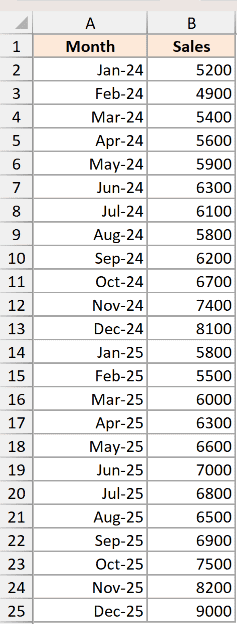
Here are the steps to create a forecast using the Forecast Sheet:
- Select both columns of your data, the dates and the values, including the headers.
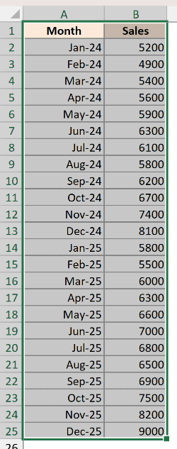
- Go to the Data tab and click Forecast Sheet in the Forecast group.

- In the Create Forecast Worksheet dialog box, set the Forecast End date to how far out you want to predict.
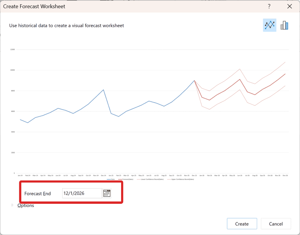
- Click Options at the bottom to set extras like the Confidence Interval and Seasonality. You can leave Seasonality on Detect Automatically.
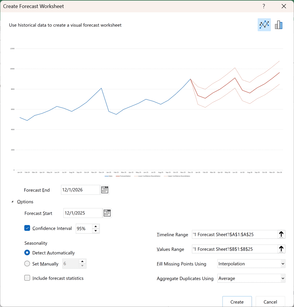
- Click Create.
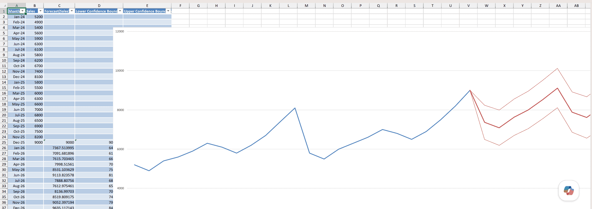
Excel adds a new worksheet with a table of your original values plus the forecast, along with a chart that shows the historical line and the predicted line together.
The forecast column also includes a lower and upper confidence bound, so you can see the likely range rather than just a single number.
Behind the scenes, the Forecast Sheet uses the FORECAST.ETS function, which is good at handling repeating seasonal patterns. You do not have to write that formula yourself, which is the whole point of this feature.
Pro Tip: The Forecast Sheet works best when your timeline has consistent intervals (one point per month, for example) and you have at least a couple of full cycles of history, like 24 months for a yearly pattern.
The Forecast Sheet is available in Excel 2016 and later, including Microsoft 365. Note that it lives in Excel for Windows, so you won’t find the same button on the Mac version.
Method 2: Using the FORECAST.LINEAR Function
If your data follows a straight-line trend and you just want a single predicted number in a cell, FORECAST.LINEAR is the function to reach for.
It draws the best-fit straight line through your existing data and tells you where that line would land at a future point.
Let me show you how it works.
Below I have sales numbers for periods 1 through 12 in two columns. Period numbers are in column A and the sales figures are in column B. I want to predict the sales for period 13.
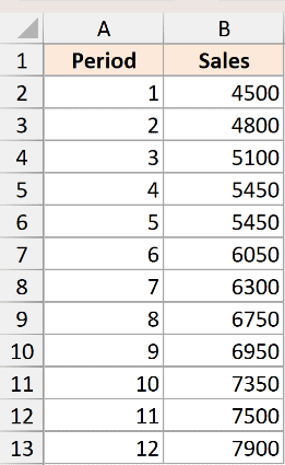
Here is the formula:
=FORECAST.LINEAR(13, B2:B13, A2:A13)
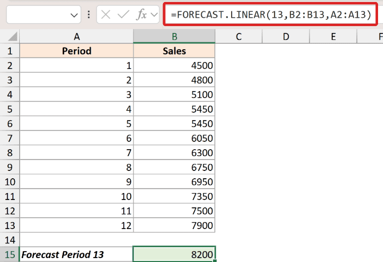
With my sample data, this returns 8200, which is the predicted sales for period 13 based on the straight-line trend.
How does this formula work?
The function takes three arguments. The first one, 13, is the x value you want a prediction for. In my case that’s the next period.
The second argument, B2:B13, is the known y values. These are the sales figures you already have.
The third argument, A2:A13, is the known x values. These are the period numbers that match each sales figure.
Excel fits a straight line to those known points and then reads off the y value at x = 13. That gives you the forecast.
A quick note on the name. You might have seen the older FORECAST function used the same way. It still works for backward compatibility, but Microsoft replaced it with FORECAST.LINEAR starting in Excel 2016, so it’s best to use the newer name in any current version.
Method 3: Using FORECAST.ETS for Seasonal Data
The straight-line approach works great for steady trends, but a lot of real data goes up and down in a repeating pattern. Think of an ice cream shop that sells more every summer and less every winter.
For that kind of data, FORECAST.ETS is a better fit because it accounts for seasonality.
This is the same engine the Forecast Sheet uses, so reach for it when you want the seasonal forecast directly in a cell instead of a whole new sheet.
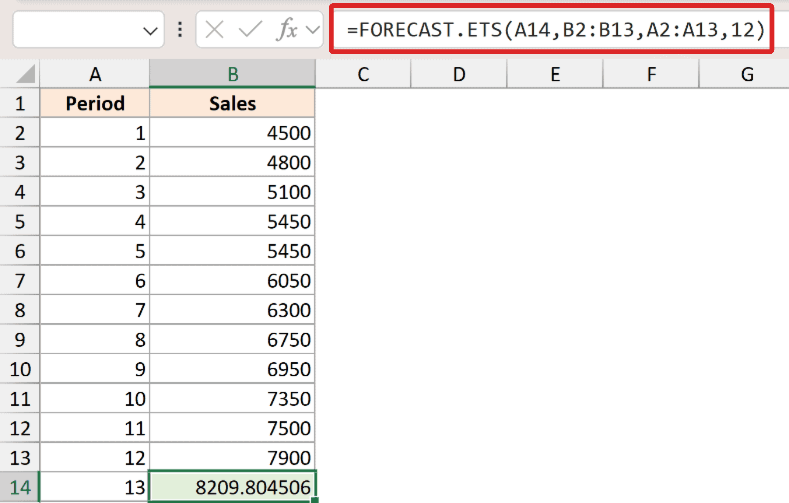
I’m using the same two columns as before, with the period numbers in A2:A13 and the matching sales figures in B2:B13, and I want a seasonal forecast for the next period in row 14.
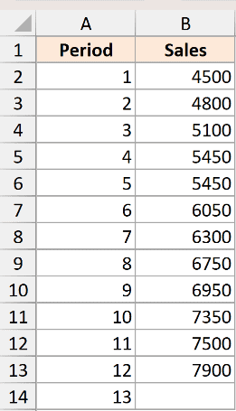
Here is the formula:
=FORECAST.ETS(A14, B2:B13, A2:A13, 12)
How does this formula work?
The first argument, A14, is the future date you want to forecast for.
The second argument, B2:B13, is your historical values, and the third argument, A2:A13, is the timeline of dates that go with them.
The last argument, 12, is the seasonality. I set it to 12 to tell Excel the pattern repeats every 12 months. You can leave this out and let Excel detect the pattern on its own.
FORECAST.ETS is available in Excel 2016 and later, including Microsoft 365.
Method 4: Using the TREND Function
The TREND function is handy when you want to project a straight-line trend across a whole range of future periods at once, rather than one value at a time.
It fits the same best-fit line as FORECAST.LINEAR, but it can return several forecasted values together.
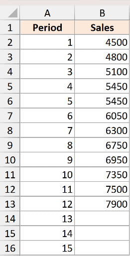
Same setup as before, with the period numbers sitting in A2:A13 and the sales figures in B2:B13. This time I want forecasts for the next three periods listed in A14:A16 all at once.
Here is the formula:
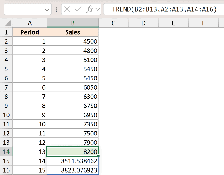
=TREND(B2:B13, A2:A13, A14:A16)
How does this formula work?
The first argument, B2:B13, is the known y values, which are your existing sales figures.
The second argument, A2:A13, is the known x values, the period numbers that match.
The third argument, A14:A16, is the new x values you want forecasts for. Excel returns a predicted value for each one.
In Microsoft 365, you can type this in a single cell and the results spill down automatically. In older versions you’d select the output range first and confirm with Ctrl + Shift + Enter.
Things to Keep in Mind
- Forecasts assume the past pattern keeps going. Excel projects whatever trend it sees forward, so a one-off event or a sudden market change won’t be predicted. Treat the number as an informed estimate, not a guarantee.
- Match the method to the shape of your data. Use FORECAST.LINEAR or TREND when the numbers move in a steady straight line, and use FORECAST.ETS or the Forecast Sheet when there’s a repeating seasonal pattern.
- Keep your timeline clean and regularly spaced. FORECAST.ETS and the Forecast Sheet expect consistent intervals, like one value per month. Gaps or uneven spacing can throw off the result.
- Give it enough history. A handful of data points is not much to learn from. For a seasonal forecast, aim for at least two full cycles so Excel can actually see the pattern.
- The old FORECAST function still works, but FORECAST.LINEAR is the current name from Excel 2016 onward. Use the newer one in any modern version.
In this article, I showed you how to forecast in Excel using the Forecast Sheet feature along with the FORECAST.LINEAR, FORECAST.ETS, and TREND functions.
I hope you found this article helpful.
Other Excel Articles You May Also Like:
