

If you want to pull the smallest, second smallest, or third smallest number out of a list, the SMALL function is what you’re looking for.
It’s the function you reach for when MIN only gives you the single lowest value and you need to go a few places past that.
In this article, I’ll show you how to use the SMALL function in Excel, from grabbing one value to spilling the bottom few numbers, sorting a list, and pulling the lowest values for just one category.
What Does the SMALL Function Do in Excel?
SMALL returns the kth smallest value from a range of numbers. You tell it which range to look at and which position from the bottom you want, and it hands back that value.
Think of it as MIN with a dial. MIN always gives you the single lowest number. SMALL lets you ask for the lowest, the second lowest, the third lowest, and so on, just by changing one number in the formula.
Syntax of the SMALL Function
=SMALL(array, k)
Arguments
- array – the range or array of numbers you want to pull a value from.
- k – the position from the bottom you want. Use 1 for the smallest, 2 for the second smallest, and so on.
A few things worth knowing before we get into the examples:
- If k is less than or equal to 0, or larger than the count of numbers in the range, SMALL returns the
#NUM!error. - If the range is empty, SMALL also returns the
#NUM!error. - SMALL only looks at numbers. It skips blank cells, text, and logical values (TRUE/FALSE) on its own, so you don’t have to clean the list first.
Example 1: Finding the Smallest Value with SMALL
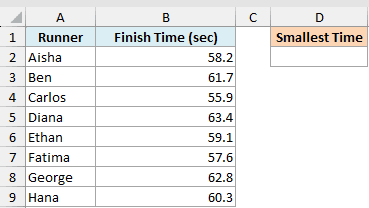
Let’s start with the simplest case. Below is a list of race finish times in seconds for eight runners, and I want to pull out the single lowest time.
Here is the formula:
=SMALL(B2:B9,1)
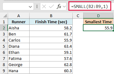
The k value here is 1, so SMALL returns the smallest number in the range, which is the fastest time.
Pro Tip: When k is 1, SMALL gives you the exact same answer as MIN. Use MIN when you only ever want the single lowest value, and switch to SMALL the moment you need the second or third lowest.
Example 2: Finding the Second or Third Smallest Value
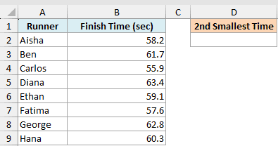
Now let’s go one step past the minimum. Here are the same eight runners and their finish times, and this time I want the second fastest time.
Here is the formula:
=SMALL(B2:B9,2)
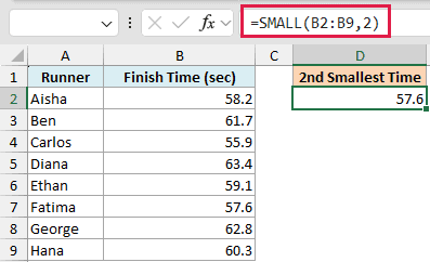
Since k is 2, SMALL skips the lowest value and returns the next one up. To get the third smallest, you’d just change the k to 3.
Example 3: Getting the Bottom 3 Values as a Spilling List
Typing a separate formula for the smallest, second smallest, and third smallest gets old fast. If you have Excel 365 or Excel 2021, you can get all three at once with a single formula that spills.
Here are the same finish times for the eight runners.
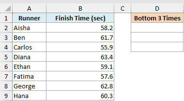
Here is the formula:
=SMALL(B2:B9,SEQUENCE(3))
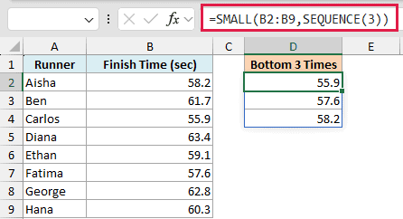
Instead of a single k, I’m feeding SMALL a small array of positions. The SEQUENCE function builds the list 1, 2, 3, so SMALL returns the smallest, second smallest, and third smallest in one go.
The result spills down into the cells below on its own. You don’t press Ctrl+Shift+Enter and you don’t drag anything down. Want the bottom five instead? Change the 3 to a 5.
Pro Tip: Make sure the cells below your formula are empty. If anything is in the way of where the result wants to spill, Excel shows a #SPILL! error instead of the values.
Example 4: Adding Up the Bottom N Values
Sometimes you don’t want to see the lowest values, you just want their total. A common case is scoring where you drop the highest results and keep the lowest few.
Below are quiz scores for eight students, and I want to add up the three lowest scores.
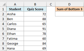
Here is the formula:
=SUM(SMALL(B2:B9,{1;2;3}))
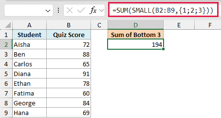
The {1;2;3} inside SMALL asks for the three smallest scores at once, and SUM adds them together into a single total.
This is an array constant, so you type the curly braces yourself. To add up the bottom five, you’d write {1;2;3;4;5} instead.
Example 5: Making SMALL Ignore Errors in the Range
SMALL happily skips blanks and text, but an error cell is different. If any cell in the range holds an error like #N/A or #DIV/0!, SMALL passes that error straight through and your formula breaks.
Below are daily sensor readings, and one cell has an #N/A error where the sensor failed. I still want the lowest valid reading.
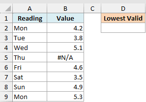
Here is the formula:
=MIN(IFERROR(B2:B9,""))
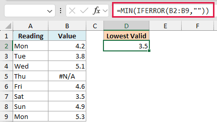
IFERROR swaps every error for an empty string, and since SMALL and MIN ignore text, the bad cell drops out of the calculation. For the smallest value, MIN reads cleaner than SMALL with a k of 1.
If you specifically need the second or third smallest while ignoring errors, use =SMALL(IFERROR(B2:B9,""),2). In Excel 365 this works as a normal formula. In older versions you confirm it with Ctrl+Shift+Enter.
Example 6: Sorting a List from Smallest to Largest with SMALL
You can use SMALL to sort a whole column of numbers in ascending order, without touching the Sort button. Below are the finish times again, and I want them laid out from fastest to slowest in a new column.
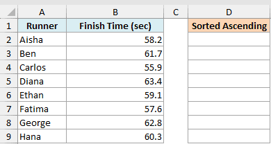
Here is the formula:
=SMALL(B2:B9,SEQUENCE(ROWS(B2:B9)))
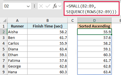
ROWS counts how many numbers are in the range, SEQUENCE builds the positions 1 through 8, and SMALL walks through them from smallest to largest. The sorted list spills down the column for you.
Pro Tip: If you only want a clean ascending sort and nothing more, the SORT function is simpler here (=SORT(B2:B9)). The SMALL version is handy when you want the sorted values to feed into a bigger formula.
Example 7: Finding the Smallest Value for One Category
Often your list has more than one group in it and you want the lowest value from just one of them. Below are delivery times in minutes along with the city each delivery went to, and I want the fastest delivery for New York only.
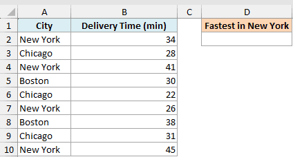
Here is the formula:
=SMALL(FILTER(B2:B10,A2:A10="New York"),1)
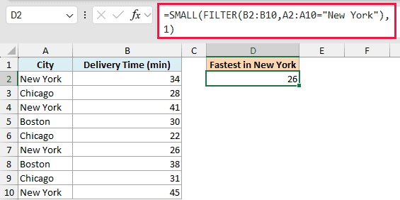
FILTER first pulls out only the delivery times for New York, then SMALL grabs the lowest one from that shorter list. Change the 1 to a 2 and you get the second fastest New York delivery.
FILTER needs Excel 365 or Excel 2021. On older versions, you’d use an array formula like =MIN(IF(A2:A10="New York",B2:B10)) confirmed with Ctrl+Shift+Enter instead.
A Few Things to Keep in Mind
- SMALL ignores blanks and text, but not errors. Blank cells and text values are skipped automatically. A
#N/Aor#DIV/0!in the range breaks the result, so wrap the range in IFERROR when the data might be messy. - Duplicates count as separate values. If two cells both hold the lowest number, SMALL with k=1 and k=2 both return that same number. It doesn’t collapse duplicates into one.
- Watch the k value. If k is 0, negative, or bigger than the count of numbers in the range, you get the
#NUM!error. - Spilling formulas need Excel 365 or 2021. The SEQUENCE and FILTER examples above use dynamic arrays. On older versions, use the per-value or Ctrl+Shift+Enter alternatives shown alongside them.
That’s how the SMALL function works in Excel, from grabbing a single low value to spilling the bottom few, summing them, sorting a list, and pulling the lowest value for one category.
It’s a small function, but once you start reaching past MIN, it earns a spot in your toolkit. I hope you found this tutorial helpful.
Other Excel Articles You May Also Like:
