

If you want Excel to tell you what kind of value is in a cell, whether blank, a number, text, or an error, the IS functions are what you need. Each one asks a simple yes-or-no question and hands back TRUE or FALSE.
“IS” is not a single function. It is a small family of them (ISBLANK, ISNUMBER, ISTEXT, ISERROR, and a few more), and they all follow the same easy pattern.
In Excel 365 you can also feed one of these a whole range and the TRUE/FALSE answers spill down the cells below.
In this article I’ll show you how to use the IS functions with real examples, from flagging empty cells to hiding lookup errors and auditing which cells hold formulas.
Follow along with the example file
IS Function Examples.xlsx
IS Functions Syntax
Each IS function takes one argument. Most test values, while ISFORMULA needs a cell or range reference and ISREF tests whether the argument is a reference.
=ISxxx(value)
- value – the cell, reference, or item you want to test. That’s the only argument any of these take.
Here are the members of the family and what each one checks:
- ISBLANK – TRUE when the value is an empty cell.
- ISNUMBER – TRUE when the value is a number (dates and times count as numbers).
- ISTEXT – TRUE when the value is text.
- ISNONTEXT – TRUE when the value is anything that is not text (including a blank cell).
- ISLOGICAL – TRUE when the value is TRUE or FALSE.
- ISERROR – TRUE for any error value (#N/A, #VALUE!, #REF!, #DIV/0!, #NUM!, #NAME?, #NULL!).
- ISERR – TRUE for any error except #N/A.
- ISNA – TRUE only for the #N/A error.
- ISREF – TRUE when the value is a valid reference.
- ISEVEN – TRUE when the number is even.
- ISODD – TRUE when the number is odd.
- ISFORMULA – TRUE when the cell contains a formula.
The IS functions work in Excel for Microsoft 365, Excel 2024, 2021, 2019, 2016, and older versions, plus Excel on the web. ISFORMULA is the one exception, added in Excel 2013.
When to Use the IS Functions
Reach for an IS function whenever you need to check a value before you act on it. Common cases:
- Flag empty cells in a form or checklist so nothing gets missed.
- Confirm a column holds real numbers and not numbers stored as text.
- Check whether a cell contains a specific word or code.
- Catch and hide errors so your reports stay clean.
- Audit a sheet to see which cells are formulas and which were typed in by hand.
Most of the time you’ll wrap an IS function inside the IF function, so the TRUE/FALSE answer turns into a helpful label or a different result.
Let me show you a few practical examples of how these work.
Example 1: Flag Empty Cells With ISBLANK
Let’s start with a simple one. ISBLANK tells you whether a cell is empty, which is handy for spotting gaps in a form.
Below is an onboarding checklist. Column A has the new hire’s name and column B shows the date they returned their signed contract. Some of those dates are still missing.
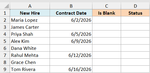
I want to check, for each row, whether the contract date is blank.
Here is the formula:
=ISBLANK(B2:B9)
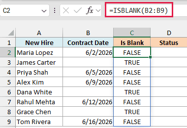
Because I fed it the whole range B2:B9 in one go, the formula spills a TRUE or FALSE down the column automatically. TRUE means that cell is empty, FALSE means it has a date.
A raw column of TRUE/FALSE isn’t very friendly, so let’s turn it into a clear label with IF.
=IF(ISBLANK(B2:B9),"Missing","Received")
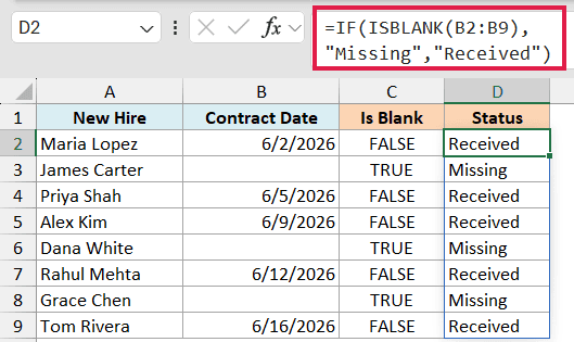
Now every empty cell reads “Missing” and every filled one reads “Received”. ISBLANK does the checking, and IF swaps in the words you actually want to see.
If you just want a headcount of how many contracts are in, the COUNTA function counts the non-empty cells in the column for you.
Pro Tip: ISBLANK only returns TRUE for a truly empty cell. A cell holding an empty string from a formula (like =””) looks blank but ISBLANK reports FALSE. For that case, test the cell length instead with =LEN(A2)=0.
Example 2: Check a Column Holds Real Numbers With ISNUMBER
Here’s a problem that trips people up all the time. Numbers pasted in from another system often come in as text, and then your SUMs quietly return the wrong total.
Below I have amounts imported into column B. A few of them look like numbers but are actually stored as text, which is hard to spot by eye.
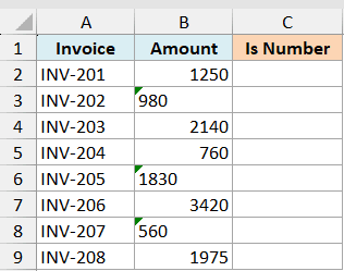
I want to check which of these values Excel actually sees as a number.
Here is the formula:
=ISNUMBER(B2:B9)
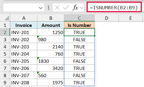
The formula spills a TRUE or FALSE for every value. Any FALSE is a number stored as text, so those are the ones you need to convert before totalling the column.
This is the reliable way to tell them apart, since a text “1250” and a real 1250 can look identical in the cell.
Pro Tip: Excel stores dates and times as numbers, so ISNUMBER returns TRUE for a real date. If it returns FALSE on something that looks like a date, that date is text and won’t work in calculations.
Example 3: Check if a Cell Contains Specific Text With ISNUMBER and SEARCH
Now let’s use ISNUMBER in a way you might not expect. Paired with SEARCH, it can check whether a cell contains a certain word or code.
Below is a list of email addresses in column A. I want to flag which ones contain “gmail” somewhere in the address.
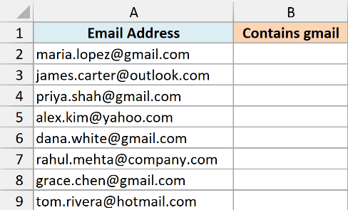
I want a TRUE next to every address that contains “gmail” somewhere inside it.
Here is the formula:
=ISNUMBER(SEARCH("gmail",A2:A9))
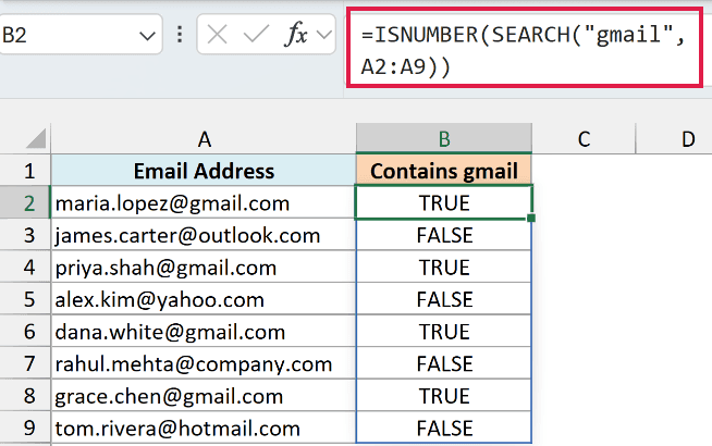
Here is how this formula works:
- SEARCH(“gmail”,A2:A9) looks for “gmail” in each address. When it finds the word, it returns the position number where it starts. When it doesn’t, it returns a #VALUE! error.
- ISNUMBER then checks that result. A position number is a number, so it returns TRUE. The #VALUE! error is not a number, so it returns FALSE.
The result spills down the column, giving you TRUE wherever “gmail” appears. This is the standard way to check if a cell contains specific text, and SEARCH ignores upper and lower case. It doesn’t verify the email’s domain or validate the address.
Example 4: Validate a Text Column With ISTEXT and ISNONTEXT
ISTEXT and ISNONTEXT are opposites, so let’s look at them together. ISTEXT is TRUE for text, and ISNONTEXT is TRUE for everything that isn’t text.
Below I have product codes in column A. These are supposed to be text labels like “SKU-204”, but a couple of rows were entered as plain numbers by mistake.
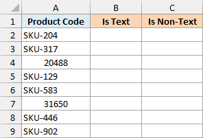
I want to confirm which entries are genuinely text.
Here is the formula:
=ISTEXT(A2:A9)
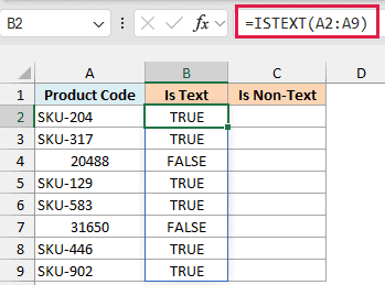
Every proper code returns TRUE, and the rows entered as numbers return FALSE. That FALSE is your flag that the entry needs fixing.
If you’d rather flag the problem rows directly, ISNONTEXT does the reverse and marks anything that isn’t text.
=ISNONTEXT(A2:A9)
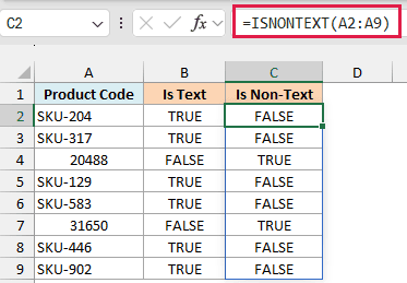
Now the numeric mistakes return TRUE. Pick whichever one reads more naturally for your check.
Pro Tip: ISNONTEXT returns TRUE for a blank cell, since an empty cell is not text. If you don’t want blanks flagged, combine it with ISBLANK, like =AND(ISNONTEXT(A2),NOT(ISBLANK(A2))).
Follow along with the example file
IS Function Examples.xlsx
Example 5: Hide Calculation Errors With ISERROR
One of the most common jobs for an IS function is catching errors so your sheet doesn’t fill up with ugly #DIV/0! and #VALUE! messages.
Below I have sales in column B and the number of orders in column C. The average value per order is sales divided by orders. The trouble is that a couple of rows have zero orders, and dividing by zero gives an error.
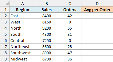
I want the average per order, but with a clean label instead of an error where orders are zero.
Here is the formula:
=IF(ISERROR(B2/C2),"No orders",B2/C2)
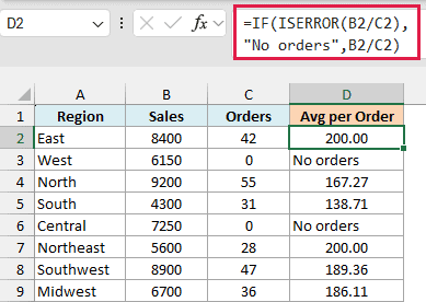
ISERROR checks whether B2/C2 produces an error. If it does, IF shows “No orders”. If it doesn’t, IF shows the actual result. So the divide-by-zero rows read “No orders” instead of #DIV/0!.
Here we keep this per-row so you can see the ISERROR check clearly. You’ll want to copy the formula down the column for each row. This label fits this numeric dataset; ISERROR would also hide unrelated errors as “No orders”.
Pro Tip: The IF plus ISERROR combo can be shortened. The IFERROR function does the same job in one step, like =IFERROR(B2/C2,”No orders”), and it only calculates B2/C2 once instead of twice.
Example 6: Handle a “Not Found” Lookup With ISNA
When a lookup can’t find a match, it returns the #N/A error specifically. ISNA is built to catch that one error and nothing else, which is useful when you want a “not found” message but still want real errors to show through.
Below I have a lookup table of product IDs and names in columns A and B. The IDs I’m searching for are in column D, and the results go in column E.
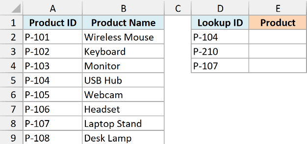
I want to return the product name, or “Not in catalog” when the ID isn’t found.
Here is the formula:
=IF(ISNA(XLOOKUP(D2,$A$2:$A$9,$B$2:$B$9)),"Not in catalog",XLOOKUP(D2,$A$2:$A$9,$B$2:$B$9))
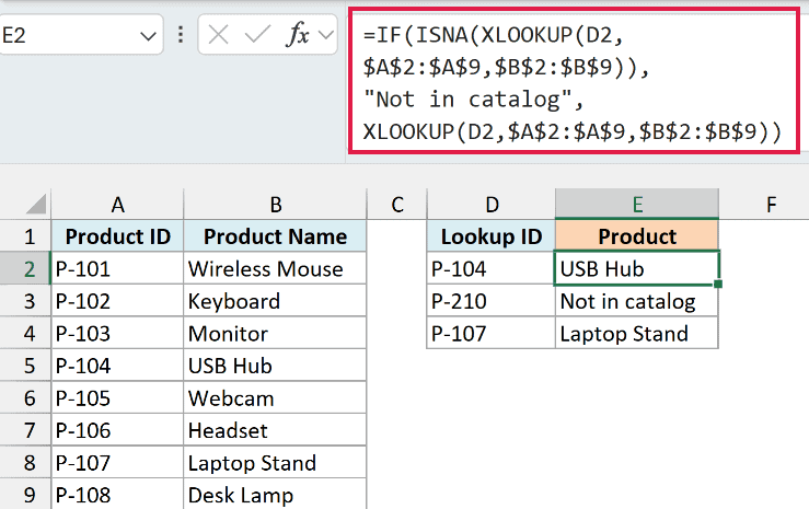
XLOOKUP returns #N/A when the ID isn’t in the table. ISNA spots that #N/A and IF swaps in “Not in catalog”. A found ID skips straight to the product name.
Using ISNA instead of ISERROR here is deliberate. Errors other than #N/A remain visible, but a matched product name containing #N/A would also become “Not in catalog”. XLOOKUP’s fourth argument handles an unfound ID more directly.
Pro Tip: XLOOKUP is available in Excel 365 and Excel 2021. On older versions, use VLOOKUP in the same pattern, like =IF(ISNA(VLOOKUP(D2,$A$2:$B$9,2,FALSE)),”Not in catalog”,VLOOKUP(D2,$A$2:$B$9,2,FALSE)).
Example 7: Classify Numbers as Even or Odd With ISEVEN and ISODD
ISEVEN and ISODD are another matched pair. One is TRUE for even numbers, the other for odd, and they’re handy for splitting a list into two groups.
Below I have employee IDs in column A. I want to assign each person to Team A or Team B based on whether their ID is even or odd.
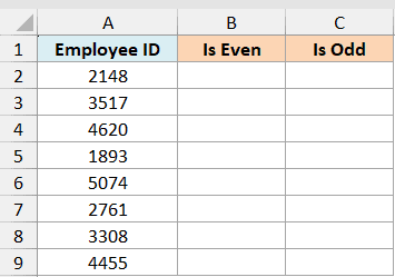
I want a quick TRUE/FALSE showing which IDs are even.
Here is the formula:
=ISEVEN(A2)
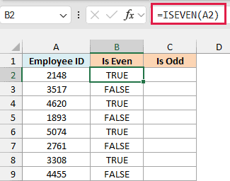
Enter it in B2 and copy it down the column, and you get a TRUE for every even ID and FALSE for every odd one. ISEVEN won’t take a plain range (=ISEVEN(A2:A9) returns #VALUE!), but in dynamic-array Excel =ISEVEN(+A2:A9) spills the results. ISODD is simply the reverse.
=ISODD(A2)
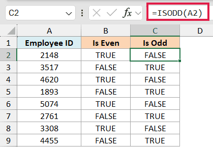
Now the odd IDs return TRUE. To turn this into team names, wrap it in IF, like =IF(ISEVEN(A2),”Team A”,”Team B”).
Pro Tip: ISEVEN and ISODD ignore anything after the decimal point, so ISEVEN(4.9) still returns TRUE because it reads the 4. ISEVEN(“2”) also returns TRUE, but ISEVEN(“abc”) gives #VALUE!.
Example 8: Audit Formulas vs Hardcoded Values With ISFORMULA
Here’s one that’s great for checking a sheet you inherited. ISFORMULA tells you whether a cell contains a formula or a typed-in value, so you can spot where someone overwrote a calculation with a hardcoded number.
Below is a small budget. Column D is meant to be quantity times price, so every cell should be a formula. But one row was typed in by hand.
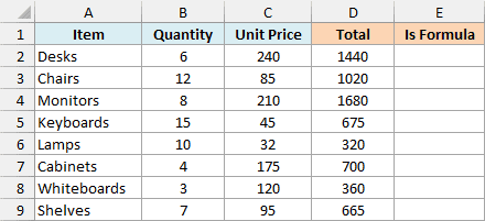
I want to see which cells in column D are actually formulas.
Here is the formula:
=ISFORMULA(D2:D9)
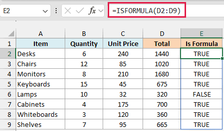
Every genuine formula returns TRUE. The row that was typed in returns FALSE, so it stands out immediately. This is a fast way to find the one hardcoded value hiding in a column of formulas.
Pro Tip: ISFORMULA and FORMULATEXT were both added in Excel 2013. On Excel 2010 or earlier, turn on Show Formulas (Ctrl + backtick) to see the formulas all at once.
Tips & Common Mistakes
A few things worth keeping in mind when you use the IS functions:
- ISNUMBER doesn’t convert text. A number in quotes, like “19”, stays text, so ISNUMBER(“19”) returns FALSE. Parity checks such as ISEVEN can convert numeric text.
- ISBLANK is stricter than it looks. It’s only TRUE for a genuinely empty cell. A formula result of “” isn’t blank to ISBLANK, so use =LEN(A2)=0 if you need to catch those too.
- Pick the right error function. ISERROR catches every error, ISNA catches only #N/A, and ISERR catches everything except #N/A. Use ISNA for lookups when you want real errors to still show.
- IFERROR is often the cleaner choice. If all you want is to replace an error with a value, IFERROR does it in one step instead of pairing ISERROR with IF.
- The spilling form needs a modern Excel. Value tests such as ISBLANK, ISNUMBER, and ISTEXT can spill for a whole range in Microsoft 365 or Excel 2021 and later. On older versions, test one cell and copy down. ISREF tests the reference itself and returns a single TRUE or FALSE.
Wrapping Up
The IS functions are small, but they save you constantly once they click. Each one asks a single yes-or-no question about a value, and you’ll mostly use them inside IF to turn that answer into a label or a safer result.
Start with the ones you’ll reach for most (ISBLANK, ISNUMBER, and ISERROR), and add the others as you run into a job that needs them.
I hope you found this tutorial helpful.
Other Excel Articles You May Also Like:
