SORT Function in Excel

If you want a sorted copy of your data that updates on its own, without clicking the Sort button every time something changes, the SORT function is what you’re after.

You hand it a range, and it gives you back a sorted version in a new spot, leaving your original data exactly where it is.

SORT is a dynamic array function. From a single formula, it spills the sorted results across the cells below.

In this article, I’ll show you how to use SORT with real examples, from a plain A-to-Z list to multi-level and horizontal sorts.

I’ll also cover keeping the header row, skipping blank cells, and pairing SORT with FILTER, UNIQUE, and TAKE.

SORT Function Syntax

Here is the syntax of the SORT function:

=SORT(array, [sort_index], [sort_order], [by_col])

• array – the range or array you want to sort. This is the only required argument.
• sort_index – optional. The column number to sort by when sorting rows, or the row number when sorting columns. It defaults to 1.
• sort_order – optional. Use 1 for ascending order (the default) or -1 for descending order.
• by_col – optional. Use FALSE to sort rows by a column (the default) or TRUE to sort columns by a row.

Only the array is required, so =SORT(A2:A10) on its own sorts that range A-to-Z down the rows.

Important: SORT works in Microsoft 365, Excel 2024, Excel 2021, Excel for the web, and current Mac versions. Excel 2019 and earlier don’t have it and show a #NAME? error.

When to Use the SORT Function

Use SORT when you need to:

• Build an alphabetical or chronological list that re-sorts itself whenever the source changes.
• Show a sorted copy of a table while the original rows stay in their entered order.
• Sort a range by a chosen column, ascending or descending.
• Apply two or more sort levels at once, each with its own direction.
• Reorder data laid out sideways by using a row as the sort key.
• Sort a list that has blank cells without ending up with zeros at the bottom.
• Keep FILTER or UNIQUE results in a predictable order for reports and dropdown sources.

One thing to be clear about up front. SORT builds a separate sorted result and never touches the original cells.

If you want to reorder the actual data in place, by color or through a dialog, that’s the Data tab’s Sort feature, which I cover in a separate guide on how to sort in Excel.

Let me show you a few practical examples of how SORT works.

Example 1: Sort a List Alphabetically

Let’s start with the simplest case, a single column of text.

Below is a list of student names in A2:A10, names like Mateo, Hana, Kwame, Ingrid, and Diego, entered in the order they joined the class.

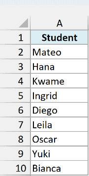
I want an A-to-Z copy of this list that re-sorts itself whenever I add or change a name.

Here is the formula:

=SORT(A2:A10)

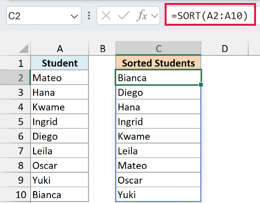
Because I only gave SORT the array, it falls back on the defaults: sort_index 1, ascending order, sorted by rows. So it sorts the single column A-to-Z.

You type the formula once and the nine sorted values spill down the cells below on their own. There’s no dragging and no filling.

Important: Leave the spill area empty. If anything blocks the cells the result needs, you get a #SPILL! error instead of the sorted list. Select the error cell to see what’s in the way.

The original list in column A stays exactly as it was. This is a fresh, sorted copy sitting wherever you put the formula.

Important: A spilled result can’t spill inside an Excel Table. If your data is in a Table, put the SORT formula in a normal range next to the table.

It’s a simple way to sort data in alphabetical order with a formula instead of the Sort button.

Pro Tip: Add a new name at the bottom of the source list and the sorted spill updates instantly to include it, in the right alphabetical spot.

Example 2: Sort Entire Dataset by Date

Here’s a more common scenario, sorting a whole dataset by one of its columns.

Below I have customer orders with the Product in column A, the Customer in column B, the Delivery Date in column C, and the Region in column D, sitting in A2:D11.

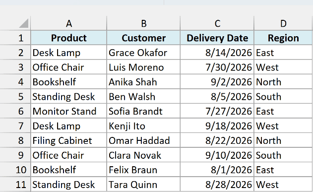
I want every row ordered from the earliest delivery date to the latest, with each order kept intact.

Here is the formula:

=SORT(A2:D11,3,1)

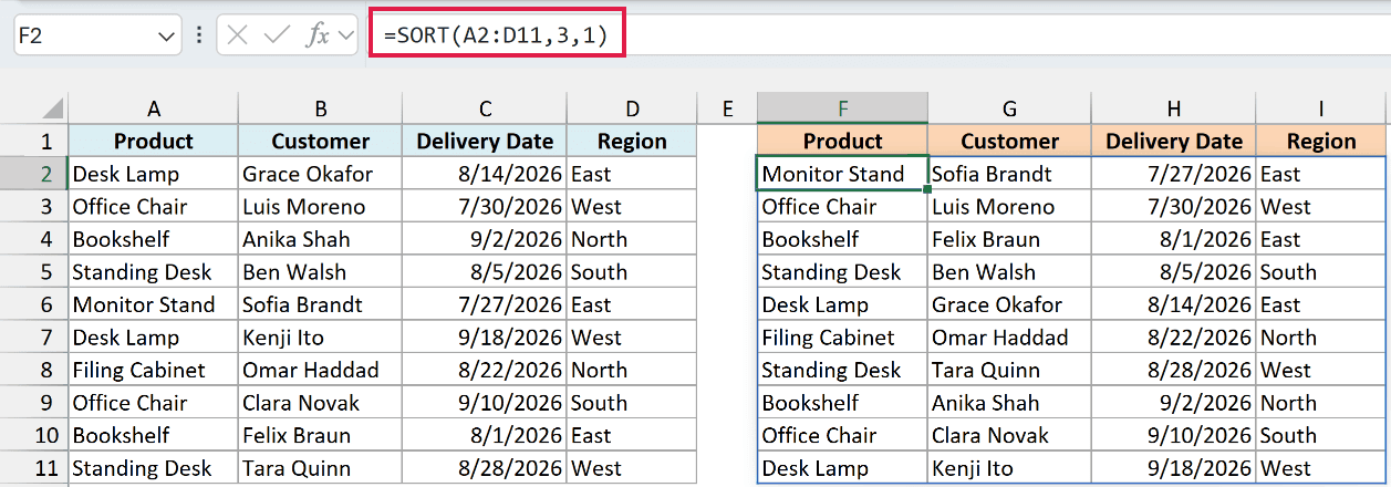
Here the sort_index of 3 points at the third column of the array, which is the Delivery Date, and the sort_order of 1 sorts it in ascending order.

Pro Tip: sort_index is the column’s position inside your array, not its column letter. If inserting or deleting columns could shift it, SORTBY with an explicit key range is safer.

The result spills as a full four-column table, and SORT moves whole rows together. Each order keeps its own product, date, and region, so the rows just change position.

Dates are stored as numbers behind the scenes, so sorting them ascending puts the earliest date first. Notice the array starts at row 2, so the header row is left out of the sort.

Important: SORT has no “my data has headers” option. Include the header row in the array and it gets sorted in with the data. Example 6 shows how to keep it.

Example 3: Sort Numbers in Ascending or Descending Order

Now let’s sort by a number instead of a date, which works the same way.

Below are gym members with the Member ID in column A, the Branch in column B, the Days Left on the membership in column C, and the Last Visit date in column D, in A2:D12.

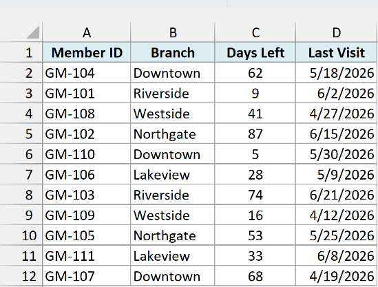
I want the members with the fewest days left at the top, so the memberships that run out first are easy to spot.

Here is the formula:

=SORT(A2:D12,3,1)

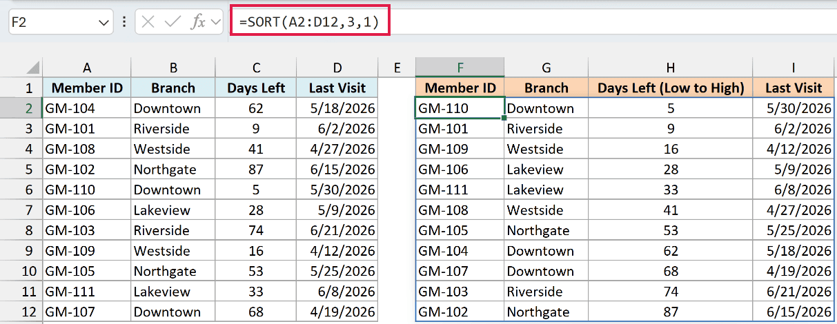
The sort_index of 3 sorts by the Days Left column, and the sort_order of 1 puts the smallest number first. The membership closest to running out ends up at the top.

To flip the order and see the members with the most days left first, change the sort_order to -1:

=SORT(A2:D12,3,-1)

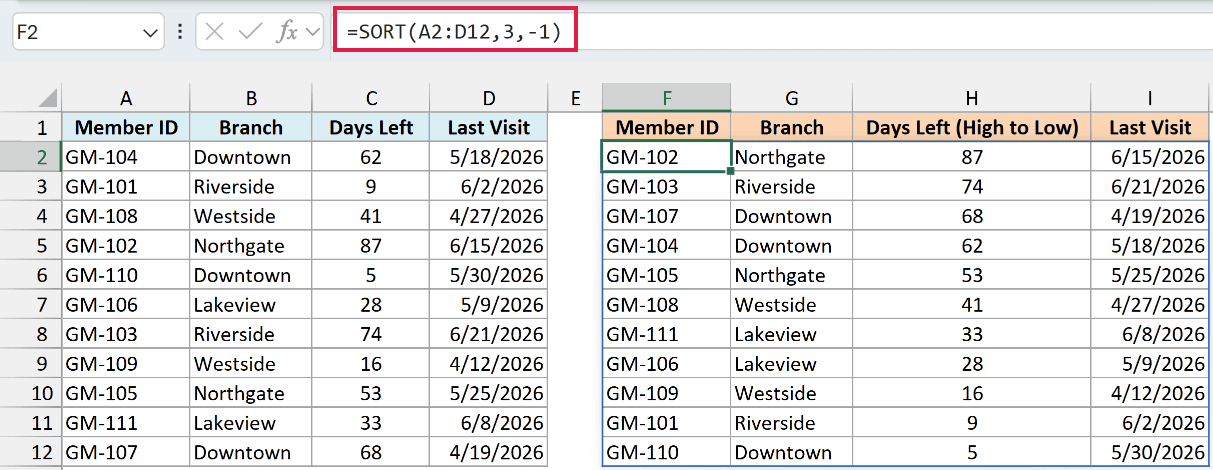
Now the largest number comes first, so the member with 87 days left sits at the top. That’s all it takes to sort largest to smallest.

Important: sort_order only accepts 1 or -1. Any other number, or a sort_index bigger than the number of columns in your array, returns a #VALUE! error.

Example 4: Sort by Multiple Columns

Let’s step it up. SORT can apply more than one sort level in a single formula.

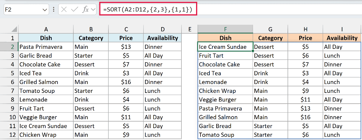
Below is a restaurant menu with the Dish in column A, the Category in column B, the Price in column C, and the Availability in column D, in A2:D12.

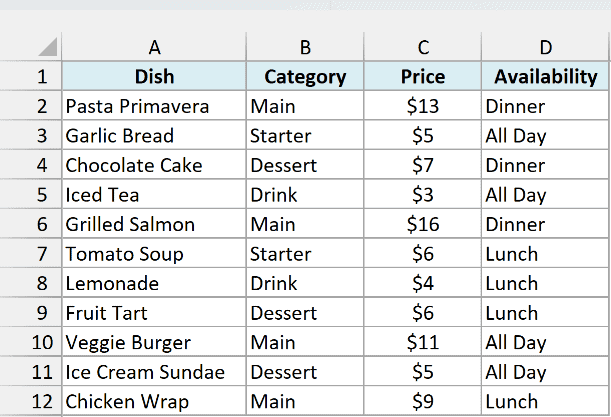
I want the dishes grouped by category alphabetically, and inside each category I want the cheapest dish first.

Here is the formula:

=SORT(A2:D12,{2,3},{1,1})

To sort on two columns, you pass an array constant to each of the two arguments:

• {2,3} for sort_index tells SORT to sort by column 2 (Category) first, then by column 3 (Price) to break ties within each category.
• {1,1} for sort_order sorts both of those ascending.

Sorting the price ascending puts the cheapest dish at the top of each category group.

Pro Tip: The two array constants must be the same length, one sort_order per sort_index. If you wanted the categories A-to-Z but the price sorted high to low, you’d use {1,-1}.

Example 5: Sort Data Left to Right Across Columns

Most data runs down in rows, but SORT can also sort sideways when your data is laid out across columns.

Below I have month labels across B1:M1 and the sales for each month across B2:M2.

I want the month columns reordered from the highest sales to the lowest, so the best months line up on the left.

Here is the formula:

=SORT(B1:M2,2,-1,TRUE)

The last argument is the key here:

• TRUE for by_col tells SORT to sort the columns rather than the rows.
• 2 for sort_index now means the second row of the array, which is the Sales row, so that’s what it sorts on.
• -1 for sort_order sorts those values from highest to lowest.

The whole two-row block spills sideways, and each month label stays glued to its own sales figure as the columns shuffle into place.

Example 6: Sort Data and Keep the Header Row

So far, every sorted result has come out without headers. Here’s how to bring the header row along.

Below is a list of hotels with the Hotel in column A, the City in column B, the Rating in column C, and the Price per Night in column D, in A1:D11.

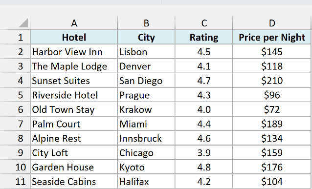
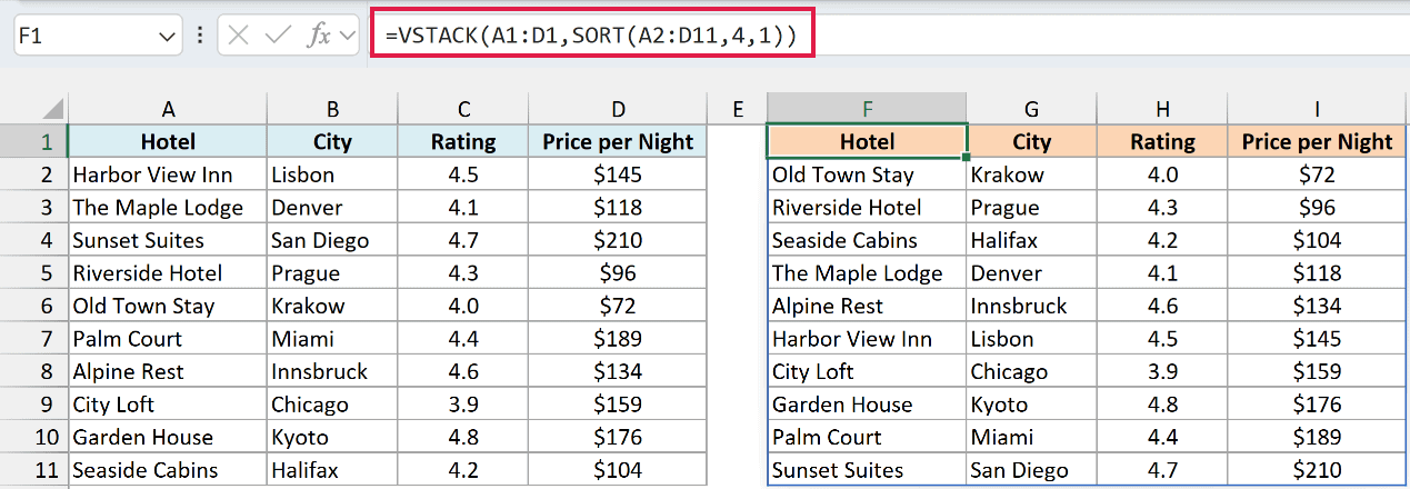
I want the hotels sorted from the cheapest night to the most expensive, with the header row sitting on top of the result.

Here is the formula:

=VSTACK(A1:D1,SORT(A2:D11,4,1))

How this formula works:

• SORT(A2:D11,4,1) sorts only the data rows by column 4, the Price per Night, with the cheapest first.
• VSTACK(A1:D1, …) stacks the header row on top of that sorted block, so both spill out as one table.

The header stays put at the top, and the rows below it re-sort on their own whenever a price changes.

Important: VSTACK needs Microsoft 365 or Excel 2024. In Excel 2021, type the headers in a row yourself and put the SORT formula in the cell just below them.

Example 7: Sort Filtered Results with FILTER

This is where SORT gets really handy. You can sort the output of another dynamic array function by nesting them.

Below are animal-shelter records with the Animal ID in column A, the Animal Type in column B, the Appointment Date in column C, and the Status in column D, in A2:D15.

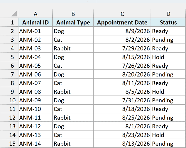
I want to show only the records marked Ready, with their appointments ordered from earliest to latest.

Here is the formula:

=SORT(FILTER(A2:D15,D2:D15="Ready"),3,1)

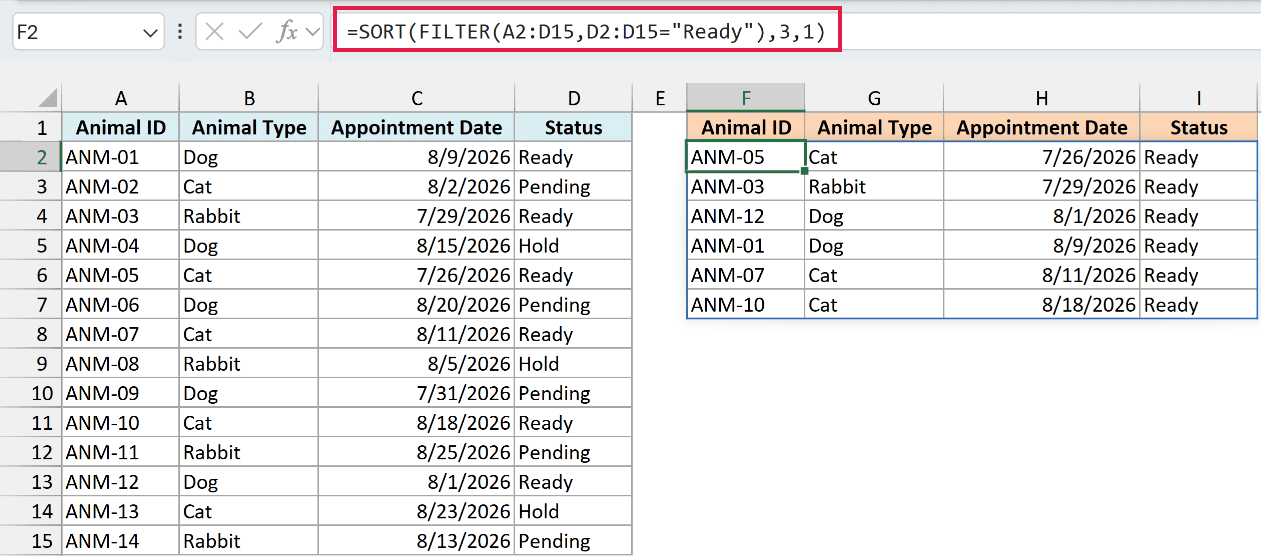
Working from the inside out, the FILTER function keeps only the rows where the Status column equals “Ready” and returns that subset as an array.

SORT then takes that filtered array and orders it by column 3, the Appointment Date, in ascending order. The final result spills as a clean, ready-only table sorted by date.

Because both are dynamic array functions, they nest neatly, and the result updates on its own as the source records change.

Example 8: Sort a List and Ignore Blank Cells

Now let’s look at a problem that shows up a lot, a list with a few blank cells in it.

Below is a shopping list in A2:A15. Some items were deleted along the way, so four of those cells are now empty.

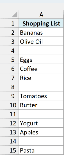
I want an A-to-Z copy of this list, with no gaps and no stray values at the end.

Let’s first see what a plain SORT does with it:

=SORT(A2:A15)

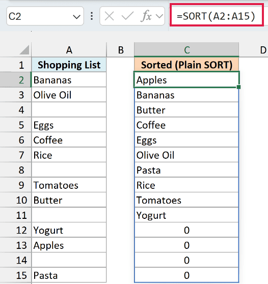
The items sort just fine, but the four blank cells land at the bottom. A spilled empty cell shows up as 0, so the list ends with four zeros.

To get rid of them, filter out the blank cells first and then sort what’s left:

=SORT(FILTER(A2:A15,A2:A15<>""))

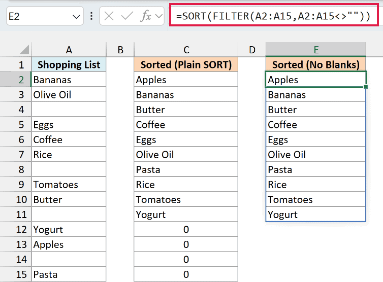
Here, FILTER keeps only the cells in A2:A15 that aren’t empty. The <>"" part means “not equal to an empty string.”

SORT then puts those ten items in A-to-Z order. There are no zeros now, and the list grows or shrinks as you add or clear items.

Example 9: Create a Sorted List of Unique Values

Another useful pairing is SORT with UNIQUE, which gives you a clean, de-duplicated list you can feed into a dropdown.

Below is an expense log where column C holds the category for each expense, in C2:C20. Categories like Food, Travel, Office, and Utilities repeat many times down the column.

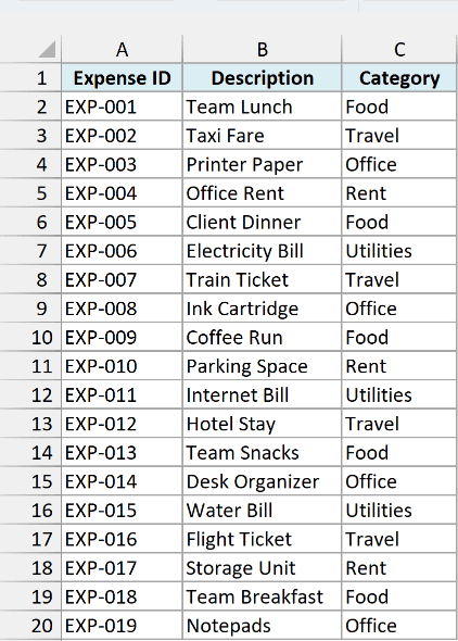
I want a clean alphabetical list of the distinct categories to use as the source for a dropdown.

Here is the formula:

=SORT(UNIQUE(C2:C20))

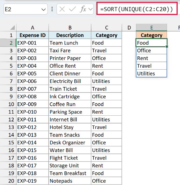
The UNIQUE function pulls out each distinct category once, and SORT wraps that list to put it in A-to-Z order.

Both spill together, so one formula gives you a sorted, duplicate-free list.

Since the result is a spill range, you can point a drop-down list at it with the spill reference operator.

If the formula sits in E2, use =$E$2# as the data validation source and the dropdown grows or shrinks as categories come and go.

Pro Tip: The # in a spill reference like E2# always points at the entire current spill, however many items it has. That’s what keeps a dropdown built on it in sync with the data.

Example 10: Get the Top Few Rows with TAKE

For the last one, let’s combine SORT with TAKE to pull just the first few rows after sorting.

Below are library book loans with the Book ID in column A, the Title in column B, the Genre in column C, and the Due Date in column D, in A2:D12.

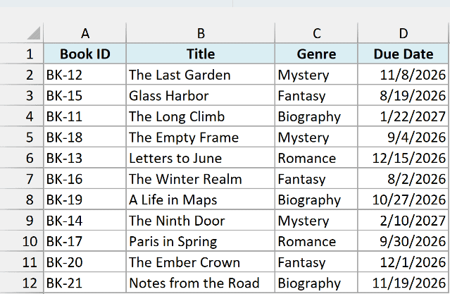
I want the three books due back soonest, and nothing else.

Here is the formula:

=TAKE(SORT(A2:D12,4,1),3)

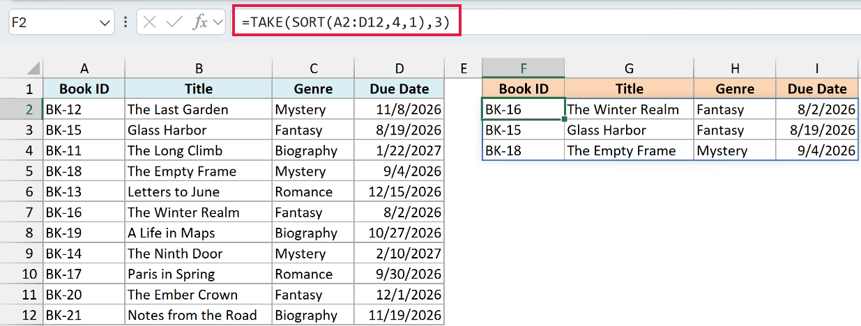
SORT does its job first, ordering the whole table by column 4, the Due Date, in ascending order so the soonest date sits at the top.

The TAKE function then grabs just the first 3 rows of that sorted array, giving you a tidy three-row “next up” list that re-sorts itself as due dates change.

Pro Tip: TAKE needs Microsoft 365 or Excel 2024. In Excel 2021, =INDEX(SORT(A2:D12,4,1),SEQUENCE(3),SEQUENCE(1,4)) returns the same top three rows.

Wrapping Up

SORT is one of those functions that quietly saves you a lot of clicking.

Once your data is set up, one formula keeps a sorted copy that updates itself, whether you’re alphabetizing a list, ordering a table by date, or sorting sideways across columns.

It gets even more useful when you nest it with FILTER, UNIQUE, and TAKE to build sorted, filtered, and trimmed lists from one formula.

I hope you found this tutorial helpful.

List of All Excel Functions

Other Excel Articles You May Also Like:

• XLOOKUP Function in Excel (12 Examples)
• SEQUENCE Function in Excel
• 20 Advanced Excel Functions and Formulas (for Excel Pros)
• Sort Dates By Month in Excel
• How to Sort Data in Excel using VBA (Range/Columns)
• How to do a Multiple Level Data Sorting in Excel
• Flip Data in Excel | Reverse Order of Data in Column/Row